Dylan Skinner Porfolio

"Correlation does not imply causation."

- Everyone at some point

This project was a joint effort by me, and my friends Jason Vasquez, Gwen Martin, and Dallin Stewart. When I say "we," I am talking about all of us together.

Neural networks have revolutionized computer science by modeling complex data relationships, yet the need to elucidate their predictions and understand underlying causality grows increasingly crucial. This project explores the integration of causal inference, traditionally rooted in statistics and philosophy, into neural networks, particularly focusing on Graph Neural Networks (GNNs) for causal modeling. Leveraging GNNs' capabilities in learning graph-structured data representations, we conduct supervised classification tasks on the LUCAS0 dataset to assess GNNs' ability to capture causal relationships and enhance interpretability and robustness. Results reveal varying accuracies across GNN architectures, with Transformer convolutional layers showing the highest performance. Comparisons against Bayesian networks, which exploit causal relationships, demonstrate superior accuracy with less training time. Moreover, employing \textbf{do}-calculus exposes GNNs' limitations in discerning precise causal relationships, underscoring the importance of causal inference for improving neural networks' predictive power. This study advocates for deeper integration of causal inference into neural network research to foster more interpretable and reliable AI systems, suggesting future exploration of diverse datasets and model architectures to validate and extend these findings.

Introduction

Neural networks are at the center of computer science research and have revolutionized our ability to model complex relationships with data. As these networks continue to proliferate in decision-making processes, output explanation and gaining a deeper understanding of the causality behind their predictions become increasingly essential. The distinction between correlation and causation is not merely philosophical; it creates the foundation for building robust, interpretable, and ethically sound AI systems.

Causal inference is a field deeply rooted in statistics and philosophy that offers a framework to disentangle cause-and-effect relationships from observed data. Traditionally, researchers have applied causal inference in fields including epidemiology, economics, and social sciences. However, integrating these ideas into the domain of neural networks presents a promising frontier with implications ranging from improving model interpretability to enhancing the fairness and accountability of AI systems.

In this project, we explore the intersection of causal inference and neural networks by focusing on the application of Graph Neural Networks (GNNs) to causal modeling. We leverage these unique capabilities of GNNs to learn representations of graph-structured data and perform a supervised classification task on the LUCAS0 dataset [7]. Our goal is to determine if GNNs can capture causal relationships within a graph and provide insights into the interpretability and robustness of these models. We also use a Bayesian network as a baseline machine learning model that leverages causal relationships to compare against the neural network.

Related Work

Integrating causal inference with neural networks has garnered significant interest in recent years. Other studies have proposed several approaches to combine the strengths from these two fields and leverage the expressive power of neural networks to model causal relationships. Koch et al. discusses ongoing work to extend causal inference to settings where confounding is non-linear, time-varying, or encoded in text, networks, and images [4]. Furthermore, Yuan et al. compared the performance of CNN's on causal data to previous methods [10].

Graph Neural Networks

The Graph Neural Networks that Mori et al. [2], originally proposed in 2005 are a class of neural networks that operate on graph-structured data. They have gained significant attention in recent years due to their versatility in handling various types of graph data, including social networks, citation networks, biological networks, and more.

Unlike traditional neural networks, which operate on grid-like structures such as images or sequences, GNNs' architectures allow them to capture and leverage the structural information present in graphs. One remarkable feature allows them to learn meaningful representations of nodes in a graph for various downstream tasks such as node classification, link prediction, and graph classification. Their ability to capture and model complex relationships in graph data makes them invaluable tools for exploring and understanding real-world phenomena represented in graph form.

In this project, we apply GNNs to a supervised classification task by training it on a labeled, tabular dataset, where we associate each graph instance (or node) with a target label.

$\textbf{do}$ Operator

The $\textbf{do}$ operator is a way to represent interventions in a causal model, i.e. the effect of an intervention on a variable. For example, consider the following model involving smoking.

If a person's fingernails $(N)$ have turned yellow, this implies a higher probability that they are a heavy smoker $(S)$ and hence have a higher probability of developing lung cancer $(C)$. However, simply dyeing someone's fingernails yellow does not impact their probability of developing lung cancer.

So, in terms of $\textbf{do}$ calculus, we can denote the process of setting a variable $N$ to have a value $\textit{yellow}$ by $\textbf{do}(N = \textit{yellow})$. We note that $$P(C \;|\;N = \textit{yellow}) \neq P(C\;|\; \textbf{do}(N=\textit{yellow})).$$ With this in mind, we now define the $\textbf{do}$ operator.

In this equation, $\text{par}(x_i)$ represents values of the parent nodes of $\text{PAR}(X_i)$ of $X_i$ in $\Gamma$. We call the probabilities on the right hand side of the above equation preintervention. Preintervention means that we use the probabilities from the original model before "doing" $X_i = x_i$.

The equation above describes how we calculate the probability of several events happening given one event has happened. What if we want to find the probability of a single event happening, given we do a single event? This scenario leads to the following corollary.

Let us now consider a basic example to see how this works. Consider the following causal diagram in Figure 1.

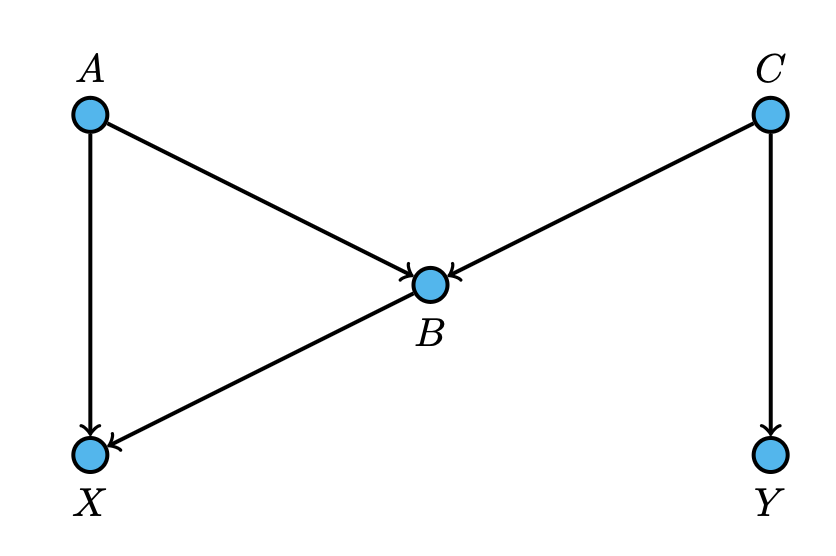
In this diagram, nodes $A$ and $C$ are both parents of $B$. So, for any values of $x$ and $b$, the above Corollary tells us that $$P(X = x \,|\, \textbf{do}(B=b)) = \sum_{\text{par}(b)}\frac{P(x, \,b, \,\text{par}(b))}{P(b\,|\, \text{par}(b))}$$ which, written out, is $$\sum_{\text{par}(b)}\frac{P(x, \,b, \,\text{par}(b))}{P(b\,|\, \text{par}(b))} = \sum_{a}\sum_{c}\frac{P(X=x\,, \, A=a\,,\, B=b \, ,\, C=c)}{P(B=b \;|\; A=a,\, C=c)}.$$ Since each node only depends conditionally on their parents, we can rewrite the expression as $$\sum_{a}\sum_{c}\frac{P(X=x\;|\; A=a\,,\, B=b)P(B=b\;|\; A=a,\, C=c)P(A=a)P(C=c)}{P(B=b \;|\; A=a,\, C=c)},$$ which simplifies to $$\sum_{a}\sum_{c}P(X=x\;|\; A=a\,,\, B=b)P(A=a)P(C=c).$$ Since there is only one instance where we are considering the probability with respect to $c$, we can further reduce this to $$\sum_{a}P(X=x\;|\; A=a\,,\, B=b)P(A=a),$$ which is our final answer.

While this introduction to the $\textbf{do}$ operator might feel a bit abstract, it is the foundation of all current research in causal inference.

Data

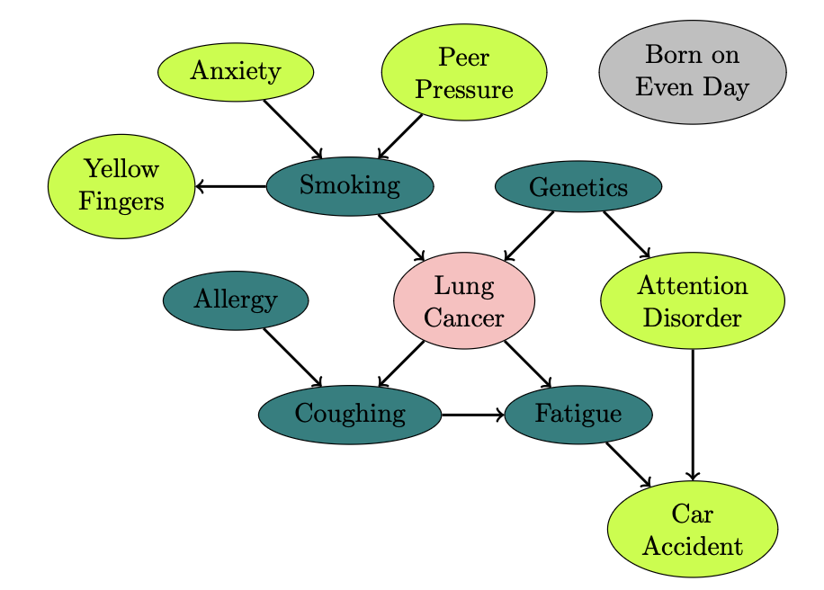
For our project, we used the LUCAS0 dataset [7], which is a synthetic toy data set with causal Bayesian networks and binary variables. The LUCAS0 dataset is a DAG with 11 nodes and 2000 training samples (see Figure 2).

We associate each node of the graph with a specific conditional probability that the creators of the dataset used to generate the data (the end of this post).

Experiments and Testing

Graph Neural Networks and Bayesian Networks perform well when handling complex structured data that consists of underlying causal relationships and do calculus operations. By examining these models more closely, we can assess their predictive power in capturing these underlying do-calculus operations. In order to do so, we train these models to predict lung cancer based on the components of the graph provided in Figure 2 and evaluate their accuracy.

Graph Convolutional Layers

We begin by training several graph neural networks with five different types of convolutional layers and performing a grid search of learning rates (0.001, 0.005, 0.01, 0.05). Each model includes a unique convolutional layer variant as at least one of seven convolutional layers. Each layer is followed by a ReLU activation function and dropout regularization, except the final layer. We describe each of these convolutional layers below.

The first type of layer we experiment with is a standard graph convolution layer acting as a control for comparison against the other layers. The other four layer types we test are Chebyshev convolution model, SAGE convolution model, GAT convolution model and a Transformer convolution model.

[1] describes a method of using Chebyshev polynomials for rapid filtering in graph neural networks. While previous methods of filtering signals in graphs require expensive computations, [1] implements Chebyshev polynomials in order to approximate kernels. These functions are easy to work with and recursively compute an orthogonal basis efficiently. The resulting combination of these Chebyshev terms can effectively represent the new filter function.

Researchers created SAGE convolutional layers to generate embeddings using node features such as various attributes, profile information and graph structure [3]>. The algorithm achieves this embedding scheme with a forward propagation algorithm that uses $K$ parameters of the model to search through the nodes. It then creates the node's embedding by sampling and aggregating the graph information. This approach provides better generalization to unseen nodes and facilitates node feature learning in a network. This algorithm is popular because of its robustness to complex node features and information.

GATConv uses attention mechanisms in order to perform node classification. [9] created this type of specialized attention layer for graph neural networks, and explained that "One of the benefits of attention mechanisms is that they allow for dealing with variable sized inputs, focusing on the most relevant parts of the input to make decisions" [9].

Researchers first adopted Graph Transformer convolution layers in an attempt to combine feature propagation and label propagation as discussed in [8]. The Transformer Convolution layer relies on a general vanilla structure of a transformer while also accounting for edge features. This layer is similar to the GATConv layer since they both use multi-headed attention.

Bayesian Network

To further investigate the ability of neural networks to learn causal relationships, we compared the results of the neural network with a Bayesian network. A Bayesian network can include causal relationships implicitly in its initialization before it fits the data. If the Bayesian network performed better than the neural networks, then we can infer that the neural networks are not able to fully grasp causal relationships. We can also infer that learning causal relationships are essential for higher accuracy when such a dependency exists in the data.

Bayesian networks, also known as belief networks or directed acyclic graphical models, are probabilistic graphical models that represent a set of variables and their conditional dependencies via a directed acyclic graph (DAG). Each node in the graph represents a random variable, and the edges between nodes represent probabilistic dependencies, indicating direct influences or causal relationships between variables.

One of the key features of Bayesian networks is their ability to model uncertainty and reason under ambiguity using Bayesian inference. By leveraging Bayes' theorem, Bayesian networks can update beliefs about variables based on observed evidence and allow for efficient probabilistic reasoning.

When comparing Bayesian networks with neural networks in learning causal relationships, Bayesian networks offer a structured framework for explicitly modeling causal dependencies between variables. We can encode prior knowledge or assumptions about causal relationships into the network structure to facilitate causal inference and reasoning. Furthermore, Bayesian networks can provide insights into causal mechanisms that may not be fully captured by neural networks alone. This source of insights is particularly salient in tasks where understanding causal relationships is crucial, such as predictive modeling in domains like healthcare or finance.

Results

Convolutional Layers and Learning Rate

While the initial accuracies provided in Table 1 appear relatively high, the performance of these models have several faults. The total percentage of lung cancer patients in this dataset is $0.7215$, so models with this level of accuracy are likely predicting ``True" each time rather than learning from the data. This behavior will cause the model to generalize poorly on other unseen data. With this in mind, both the standard and Chebyshev convolution yield insignificant results. The Transformer convolution provides the most accurate results at the expense of longer training time.

Table 1: Models by Convolutional Layers and Learning Rates

Convolutional Layers	Learning Rates
	0.001	0.005	0.01	0.05
Standard Graph Convolution	0.725	0.8325	0.725	0.725
Chebyshev Convolution	0.721	0.725	0.725	0.658
SAGE Convolution	0.8675	0.8575	0.865	0.725
GAT Convolution	0.8125	0.85	0.855	0.725
Transformer Convolution	0.8625	0.875	0.8775	0.8675

Table 2: Models by Convolutional Layers and Average Training Times

Convolutional Layers	Avg Training Time (s)
Standard Graph Convolution	0.98
Chebyshev Convolution	0.713
SAGE Convolution	12.457
GAT Convolution	9.982
Transformer Convolution	9.189

Bayesian Networks

For the Bayesian network, we initialized the model with the causal relationships on the dataset defined above, split the data randomly into $80\%$ training data and $20\%$ test data, then fit the model on the training data, which took $0.09$ seconds. The model was able to predict cancer with $86.25\%$ accuracy on the test set, beating every GNN we tested except for the Transformer models.

Evaluating Models with $\textbf{do}$ Calculus

Let's consider the following conditional probabilities with $\textbf{do}$ operators applied: \[ \begin{aligned} P(\text{LC} = \text{T} \;&|\; \mathbf{do}(\text{YF} = \text{T})), \\ P(\text{LC} = \text{T} \;&|\; \mathbf{do}(\text{PP} = \text{T})), \\ P(\text{LC} = \text{T} \;&|\; \mathbf{do}(\text{A} = \text{T})), \\ P(\text{LC} = \text{T} \;&|\; \mathbf{do}(\text{AD} = \text{T})), \\ P(\text{LC} = \text{T} \;&|\; \mathbf{do}(\text{CA} = \text{T})), \\ \end{aligned} \] where LC is lung cancer, YF is yellow fingers, PP is peer pressure, A is anxiety, AD is attention disorder, and CA is car accident. We note that we chose this probability because it does not involve any variables that are in the Markov blanket of our target variable. Thus, we should expect that there is very little predictive power in this probability.

Following the $\textbf{do}$ calculus algorithm, we write $P(\text{LC} = \text{T} \;|\; \textbf{do}(\text{YF} = \text{T}))$ (using the corollary) as \[ \begin{equation} P(\text{LC} = \text{T} \;|\; \textbf{do}(\text{YF} = \text{T})) = \sum_{s\in\{T, F\}} \frac{P(\text{YF} = \text{T},\, \text{LC} = \text{T},\, \text{S} = s)}{P(\text{YF} = \text{T}\,|\, \text{S} = s)}, \label{yf1} \end{equation} \] where $\text{S}$ is smoking. Since the Lung Cancer node has Smoking and Genetics as parents, and Smoking has parent Anxiety and Peer Pressure (see Figure 2), we can write the above equation to \[ \begin{equation} \sum_{S, G, A, PP}\frac{P(\text{YF} =\text{T}\;|\; \text{S}) P(\text{LC} = \text{T}\;|\; \text{S},\, \text{G}) P(\text{G}) P(\text{S}\;|\;\text{A},\, \text{PP}) P(\text{A})P(\text{PP})} {P(\text{YF} = \text{T}\;|\; \text{S})}. \label{yf2} \end{equation} \] where each $\text{S},\text{A}, \text{G}, \text{PP}$ is in terms of $\{T, F\}$.

Since not every term is in terms of every variable, we can rewrite the above equation as \[ \begin{align*} &=\sum_{S} \frac{P(\text{YF} = T\,|\, S)}{P(\text{YF} = T\,|\, \text{S})} \Biggl(\sum_{G} P(\text{LC} = \text{T}\,|\, \text{S}, \text{G})P(\text{G})\Biggr) \Biggl(\sum_{A} P(\text{A}) \Bigl(\sum_{\text{PP}}P(\text{S}\,|\, \text{A}, \text{PP})P(\text{PP})\Bigr) \Biggr) \\ &=\sum_{S}\Big(\sum_{G} P(\text{LC} = \text{T}\,|\, \text{S}, \text{G})P(\text{G})\Big) \Biggl(\sum_{A} P(\text{A}) \Bigl(\sum_{\text{PP}}P(\text{S}\,|\, \text{A}, \text{PP})P(\text{PP})\Bigr) \Biggr).\label{yf3} \end{align*} \] Using the probabilities from Table 5 on the above equation we get \[ \begin{equation*} P(\text{LC} = \text{T} \;|\; \textbf{do}(\text{YF} = \text{T})) = 0.7363 \end{equation*} \]

Table 3: The resulting probabilities of the do statements found in the above equation.

do Statements	Probabilities
\( P(\text{LC} = \text{T} \mid \mathbf{do}(\text{A} = \text{T})) \)	0.5158
\( P(\text{LC} = \text{T} \mid \mathbf{do}(\text{S} = \text{T})) \)	0.8639

These probabilities are what we expect based on the causal diagram. For example, the probability of cancer given $\textbf{do}$(YF = T) is hardly higher than the probability of lung cancer on its own. This helps us understand that while cancer patients are more likely to have yellow fingers, yellow fingers themselves do not cause cancer. However the probability of cancer given $\textbf{do}$(S = T) is much higher, implying that smoking does cause cancer.

We compare these probabilities to the probability output by our GNN in Table 4. To calculate these probabilities, we took a data point with False for every feature except for one feature artificially set to True, and then passed this data point through our model. The discrepancy in the probabilities seems to imply that our neural network was unable to pickup on causality, as it assumed that everyone with yellow fingers has cancer (even absent smoking).

The resulting probabilities of the do statements running the data points through the Transformer model with a learning rate of 0.01 as seen above.

do Statements	Probabilities
\( P(\text{LC} = \text{T} \mid \mathbf{do}(\text{YF} = \text{T})) \)	1.000
\( P(\text{LC} = \text{T} \mid \mathbf{do}(\text{A} = \text{T})) \)	0.1329
\( P(\text{LC} = \text{T} \mid \mathbf{do}(\text{S} = \text{T})) \)	0.9565

Conclusion

This project seeks to examine how neural networks can be used to perform do-calculus and causal inference. Graph neural networks have gained significant popularity in their ability to handle complex relationships and capture meaningful node representations. These networks achieve successful results in both computational efficiency and accuracy, with a Transformer convolutional layer model leading in performance. Bayesian networks also prove that a model that understands the causal relationships between the data can outperform most neural networks in much less time. Furthermore, using $\textbf{do}$ calculus we conclude that neural networks are unable to pickup on the exact nature of causal relationships. These results indicate that the field of causal inference is very important in neural networks and the better that neural networks can understand causal relationships, the higher the predictive power.

We recognize that there is significant room for improvement especially with a topic as complicated as causal inference in deep learning. For future work, we hope to experiment with a wider variety of datasets to explore how other graphical relationships perform with our models. Given that our testing is confined to this dataset and lacks sufficient validation across other graphs and model performances, we suggest that future work couple these results with other reliable studies in making important claims such as lung cancer detection.

Citations

1. Defferrard, Michaël, Xavier Bresson, and Pierre Vandergheynst. "Convolutional Neural Networks on Graphs with Fast Localized Spectral Filtering." 2017. Paper link.
2. Gori, Marco, Gabriele Monfardini, and Franco Scarselli. "A new model for learning in graph domains." Proceedings of the International Joint Conference on Neural Networks, vol. 2, 2005, pp. 729–734. DOI: 10.1109/IJCNN.2005.1555942.
3. Hamilton, William L., Rex Ying, and Jure Leskovec. "Inductive Representation Learning on Large Graphs." 2018. Paper link.
4. Koch, Bernard, et al. "Deep Learning of Potential Outcomes." CoRR, vol. abs/2110.04442, 2021. arXiv: 2110.04442.
5. Koller, Daphne, and Nir Friedman. Probabilistic Graphical Models: Principles and Techniques. MIT Press, 2009.
6. Pearl, Judea. "Causal Inference in Statistics: An Overview." Statistics Surveys, vol. 3, 2009, pp. 96–146. DOI: 10.1214/09-SS057.
7. Research Group for Lung Cancer Analysis. "LUCAS (LUng CAncer Simple set) Dataset." ETH Zurich Causality and Machine Learning Group, 2020. Dataset link.
8. Shi, Yunsheng, et al. "Masked Label Prediction: Unified Message Passing Model for Semi-Supervised Classification." 2021. Paper link.
9. Velicković, Petar, et al. "Graph Attention Networks." 2018. Paper link.
10. Yuan, Ye, Xueying Ding, and Ziv Bar-Joseph. "Causal inference using deep neural networks." CoRR, vol. abs/2011.12508, 2020. arXiv: 2011.12508.