Feature Selection Using $L^1$ Regularization and Stepwise Feature Removal
"It's better to enjoy life - selection is a temporary thing."
- Shreyas Iyer
The goal of machine learning is to find the best possible model for a specific problem. Typically, finding the best possible model for a specific problem ends up being nothing more than trying a bunch of different models, fiddling about with different hyperparameters, and seeing which performs the best. One additional tool that a data scientist can use to boost their model success is feature selection. In this article, we will explore two different ways to performs feature selection, namely using $L^1$ regularization and stepwise feature removal. We will also discuss how $L^1$ regularization often out performs stepwise feature removal.
Note: In this article we will be using $L^1$ regularization for linear regression and the Akaike Information Criterion (AIC) and Bayesian Information Criterion (BIC) for stepwise feature removal. If these terms are unfamiliar to you, then I suggest you read my articles on linear regression and $L^1$ regularization found here, and my article on AIC and BIC found here.
What Is Feature Selection?
Before talking about how to perform feature selection, I feel it is important to talk about what feature selection is. Feature selection is the process of selecting a subset of features from a larger set of features to use in a model, noting that each of these feature subsets will give you a different model. We can use various measures of model performance to determine which feature subset is best.
If the number of features in a dataset is small, we can simply try all possible subsets of features and choose the one that gives us the best model performance. However, if the number of features is large, then this becomes computationally infeasible since the number of feature subsets is $2^F$ where $F$ is the number of features.
The ultimate goal of feature selection is to reduce the number of features used in a model (i.e., reduce model complexity), while still maintaining a high level of model performance. This is important because it can help us avoid overfitting, and can help us build models that are more interpretable, if that is important to you.
Example Data For This Tutorial
Before getting into the data, make sure you have the following libraries installed and loaded.
import pandas as pd
import numpy as np
from statsmodels.api import sm
In this tutorial, we will be using the Auto MPG from the UC Irvine machine learning repository. This dataset contains information about different cars, such as the number of cylinders, the weight, the horsepower, and we will use it to predict the miles per gallon (mpg) of the car.
To load in this data in Python we first install the ucimlrepo library. To do this, first make sure it is installed by running
!pip install ucimlrepo
Then, we can load in the data by running
# Import the dataset
from ucimlrepo import fetch_ucirepo

# fetch dataset
auto_mpg = fetch_ucirepo(id=9)

# data (as pandas dataframes)
X = auto_mpg.data.features
y = auto_mpg.data.targets
By running auto_mpg.variables, we can get a quick look at the variables in this dataset.
auto_mpg.variables
>>>        name     role         type   missing_values
0  displacement  Feature   Continuous               no
1           mpg   Target   Continuous               no
2     cylinders  Feature      Integer               no
3    horsepower  Feature   Continuous              yes
4        weight  Feature   Continuous               no
5  acceleration  Feature   Continuous               no
6    model_year  Feature      Integer               no
7        origin  Feature      Integer               no
8      car_name       ID  Categorical               no
Note: Running auto_mpg.variables will not give this exact output. I removed some of the columns I deemed unnecessary for the sake of brevity.
(All of this is taken from the Import In Python button found on UC Irvine's page for the auto-mpg dataset.)
Now that we have the data loaded in, we also need to perform a little bit of feature engineering. Firstly, we notice that the origin
column is an integer, but when you look at the data, it is actually a categorical variable with integer values, specifically taking on the values
of $1$, $2$, and $3$, where $1$ is the US, $2$ is Europe, and $3$ is Asia. It is important that we one-hot encode this to avoid our model taking
the numerical proxy of the origin as anything other that nominal data. Here is the code that will do that.
# Change the values of the origin column to represent the country of origin as strings: 'US', 'Europe', and 'Asia'
X['origin'] = X['origin'].replace({1: 'US', 2: 'Europe', 3: 'Asia'})

# One-hot encode the origin column
X = pd.get_dummies(X, columns=['origin'], drop_first=True)
Remember to use drop_first=True to avoid creating any sort of linear dependence in the data.
We also see that the horsepower column is missing some values. Running X['horsepower'].isna().sum(), we get that there are
$6$ missing values. Since this is a small number of missing values, we can simply drop these rows. Before doing that, we need to get the rows that have the missing values, so we can
make sure to drop them from $y$. We can do this by running nan_indices = X[X.horsepower.isna()].index. Once that is done, we can drop those rows from $X$ and $y$ by running
X = X.dropna(), and y = y.drop(nan_indices).
The model we will be using for this article will be a simple linear regression model from statsmodels. Recall that when using
statsmodels for linear regression, we need to add a constant column manually. We can do this by running X = sm.add_constant(X).
Now that any necessary feature engineering is complete, we will now begin feature selection.
Stepwise Feature Removal
Stepwise feature removal is a simple, yet effective, way to perform feature selection. The idea is to start with all of the features, and then remove one feature at a time, each time fitting a model and evaluating the model performance. We then choose the model that gives us the best performance. To do this, follow these simple steps:
- Fit a model using all of the features.
- Compute the AIC and/or BIC.
- Identify a feature with a high p-value and a $95\%$ confidence interval that contains $0$.
- Drop the feature.
- Refit the model without the feature and recompute the AIC and/or BIC.
- If the AIC and/or BIC has dropped significantly, permanently drop the feature. Otherwise, add the feature back in and go back to step 3.
- Repeat steps $3-6$ until the AIC/BIC stops improving or there are no other features with a large p-value.
With this process now defined, let's see how we can implement it in Python. First, we need to define a function that will fit a model by doing
# Fit the model
model = sm.OLS(y, X).fit()
Once our model is fitted, we can use the .summary() method to get all the information we need to perform steps $3-6$ of stepwise feature removal.
Running model.summary() gives us the following output.
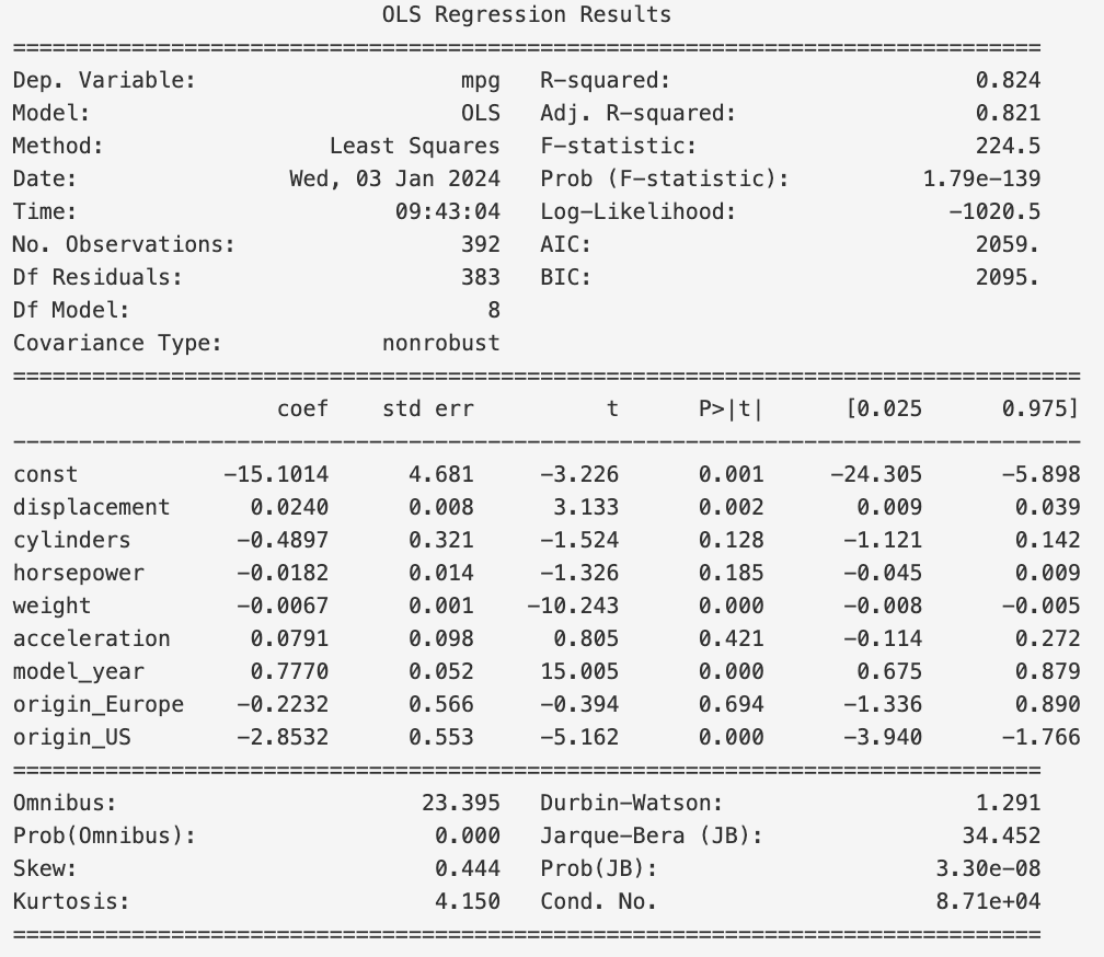
First, note the AIC and BIC. We see that they have values of $2059$ and $2095$, respectively. These are the values we will use to compare models.
Next, looking at the P>|t| column, we see that the origin_Europe feature has a p-value of $0.694$ and contains $0$
in its $95\%$ confidence interval. This means that we can drop this feature. To do this, we simply run X1 = X.drop('origin_Europe', axis=1).
(Note, we set this operation equal to X1 so we do not overwrite the original X dataframe.)
Once we have dropped the feature, we can refit the model and call model.summmary() again (remember to use X1 instead of X).
This yields
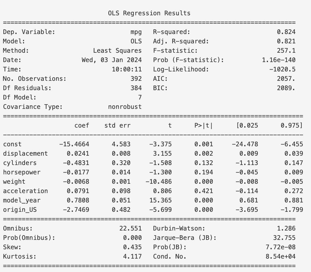
We note that the AIC and BIC have decreased from $2059$ and $2095$ to $2057$ and $2089$, respectively.
This means that we have improved our model by dropping the origin_Europe feature, so we will not add it back in.
We now select the next feature to drop. Looking at the P>|t| column, we see that the acceleration feature has a p-value of $0.421$ and contains $0$
in its $95\%$ confidence interval. This means that we can drop this feature. To do this, we simply run X2 = X1.drop('acceleration', axis=1). Refitting and calling
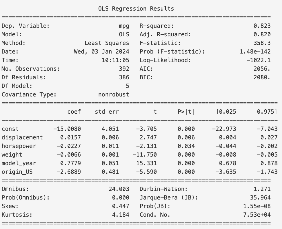
model.summary() again yields
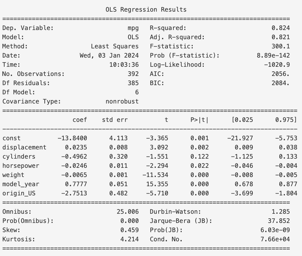
Since the AIC and BIC have decreased from $2057$ and $2089$ to $2056$ and $2084$, respectively, we have improved our model by dropping the acceleration feature, so we will not add it back in.
However, we notice that the decrease in AIC and BIC is less than the previous decrease. This means that we are not improving our model as much as we were before. This is a sign that we are nearing the end of our feature selection.
Finally, we select the next feature to drop. Looking at the P>|t| column, we see that the cylinders feature has a p-value of $0.122$ and contains $0$
in its $95\%$ confidence interval. This means that we can drop this feature. To do this, we simply run X3 = X2.drop('cylinders', axis=1). Refitting and calling
model.summary() again yields
We can see that the AIC has not changed, and the BIC has decreased from $2084$ to $2080$. This is not a very significant change, especially when
you remember that BIC penalizes model complexity more than AIC, so it makes sense that removing a feature (i.e., reducing model complexity) would
have a larger effect on BIC than AIC. This tells us that removing the cylinders feature is up to us. If we want a simpler model, then we can remove it.
If we want a more complex model, then we can keep it. In our case we will keep it.
Now that we have gone through the process of stepwise feature removal, we can calculate the mean-squared error (MSE) of our final model and compare it with
the MSE of the inital model. To do this, we first create a train_test_split of our data and then fit the initial model and the final model.
# Perform train test split
from sklearn.model_selection import train_test_split
X_train, X_test, y_train, y_test = train_test_split(X, y, test_size=0.2, random_state=334)
y_test = y_test.values

# Train the first model, and get the MSE on the test set
model = sm.OLS(y_train, X_train).fit()
y_pred = model.predict(X_test).values
mse = np.mean((y_pred - y_test)**2)
print(f'MSE when using all features:         {mse}')

# Now, remove the features we decided weren't useful through stepwise feature removal, and get the MSE on the test set
X_train = X_train.drop(['origin_Europe', 'acceleration', 'cylinders'], axis=1)
X_test = X_test.drop(['origin_Europe', 'acceleration', 'cylinders'], axis=1)
model = sm.OLS(y_train, X_train).fit()
y_pred = model.predict(X_test).values
mse = np.mean((y_pred - y_test)**2)
print(f'MSE when using only useful features: {mse}')
The output of this code is
>>> MSE when using all features:         99.67098477764772
>>> MSE when using only useful features: 98.94744747911336
Thus, we can see that our final model performs slightly better than our initial model. This is a good sign that our feature selection was successful!
$L^1$ Regularization Feature Selection
Now that we have seen how to perform feature selection using stepwise feature removal, let's see how to perform feature selection using $L^1$ regularization.
To do this, we will be using the LassoLarsIC model from sklearn.linear_model, so make sure you import that.
from sklearn.linear_model import LassoLarsIC
The LassoLarsIC function is a powerful tool for performing feature selection using $L^1$ regularization.
Recall that $L^1$ regularization introduces a penalty term based on the absolute values of the regression coefficients,
encouraging sparsity in the model by driving some coefficients to exactly zero. LassoLarsIC, short for Least
Angle Regression with AIC/BIC criterion, combines the LARS (Least Angle Regression) algorithm with the AIC or BIC, which, as we know help in
selecting the optimal subset of features by balancing model complexity and goodness of fit. LassoLarsIC sequentially adds features
to the model, monitoring the AIC/BIC at each step, and stops when the chosen criterion is optimized. This makes it an effective method
for automatic feature selection, especially in high-dimensional datasets where the number of features is large relative to the number
of observations.
Using LassoLarsIC is really quite simple. First, we need to create an instance of the model. We can do this by running
lars_model = LassoLarsIC(criterion='bic', normalize=False)
Note that we are choosing to evaluate our model based on the BIC criterion. We could also choose to use the AIC criterion
by simply replacing 'bic' with 'aic'.
Next, we fit our model. We will fit it with the same X_train and y_train that we used for stepwise feature removal so we can
compare the results with more accuracy.
lars_model.fit(X_train, y_train.values.reshape(1, -1)[0])
We see that instead of using y_train directly, we need to reshape it. This is because y_train is a pandas series
(and therefore a column vector), and LassoLarsIC expects a row vector. Using y_train.reshape(1, -1)[0] will convert
the column vector to a row vector.
Now that we have fit our model, we can see which values of $\alpha$ were used and the corresponding BIC values by running
# Get the results from the model
results = pd.DataFrame(
    {
        "alphas": lars_model.alphas_,
        "BIC criterion": lars_model.criterion_,
    }
).set_index("alphas")
print(results)
The output of this code is
             BIC criterion
alphas
5791.332580    3181.170871
23.835366      1837.591358
15.655978      1838.232508
8.145562       1831.269152
2.384037       1674.376395
0.663504       1660.903465
0.295187       1665.666492
0.232070       1662.522325
0.188430       1663.228888
0.033225       1655.087183
0.000000       1659.478067
Now, in our case we see that the optimal value of $\alpha$, according to the BIC, is $0.033225$.
We can see which features the model kept by running model.coef_. This gives us
lasso_model = Lasso(alpha=0.033225).fit(X_train, y_train.values.reshape(1, -1)[0])
print(lars_model.coef_)
>>> [ 0.02359115, -0.61367486, -0.01471611, -0.00695722,  0.04982891, 0.74492259,  0.        , -2.30763917]
This tells us that the seventh features was dropped (origin_Europe), and the remaining features were kept. If we
compute the MSE of this model and a regular linear regression model, we get
from sklearn.linear_model import LinearRegression
lasso_no_alpha = LinearRegression().fit(X_train, y_train.values.reshape(1, -1)[0])

# Get the MSE on the test set for each model
y_pred_no_alpha = lasso_no_alpha.predict(X_test)
y_pred_opt_alpha = lars_model.predict(X_test)

mse_no_alpha = np.mean((y_pred_no_alpha - y_test)**2)
mse_opt_alpha = np.mean((y_pred_opt_alpha - y_test)**2)

print(f'MSE when alpha=0:         {mse_no_alpha}')
print(f'MSE when alpha=0.033225:  {mse_opt_alpha}')
The output of this code is
>>> MSE when alpha=0:         99.6709847776471
>>> MSE when alpha=0.033225:  98.75552193526808
If we recall, the MSE of our stepwise feature removal model was $98.94744747911336$. This means that our $L^1$ regularization model performs slightly better than our stepwise feature removal model.
This brings up an important point. In general, $L^1$ regularization often outperforms stepwise feature removal in linear regression due to its automatic and continuous shrinkage of less important features. $L^1$ regularization optimizes the model globally, providing a more robust approach to feature selection by considering all features simultaneously. It effectively reduces overfitting, handles multicollinearity better, and leads to sparser models with better generalization performance compared to the stepwise feature removal method.
Conclusion
In this article, we explored two different ways to perform feature selection, namely using $L^1$ regularization and stepwise feature removal. We also discussed how $L^1$ regularization often out performs stepwise feature removal. My hope is that you now understand how you can improve your machine learning models by performing feature selection, specifically using $L^1$ regularization. If you want to see the code used in this article, you can find it on my Github. If you want to read a paper that me and some of my friend wrote that used $L^1$ regularization for feature selection, you can find it here.