Dylan Skinner Blog

"Nature abhors a gradient."

- Eric Schneider

Gradient Boosting, a powerful ensemble learning technique, is an important topic in machine learning and is the foundation of several powerful models. This sophisticated method combines the strengths of decision trees with a meticulous optimization process, leveraging the principles of boosting to sequentially improve the accuracy of weak learners. In this blog post, we'll discuss the math of gradient boosting, exploring its inner workings and understanding how it stands out among ensemble methods. We'll also shed light on AdaBoost, a version of gradient boosting, and draw comparisons between gradient boosting and random forests through a practical Python example. By the end of this journey, you'll gain a deeper insight into the mechanics of gradient boosting and its practical implications.

Why Boosting

In my previous blog post about decision trees, I mentioned the building an optimal decision tree is an NP-hard problem and how using the standard greedy method of building trees can easily overfit the data. One solution to improving decision trees is by combining bagging and attribute bagging in random forests. While incredibly powerful, random forests can still overfit the data and are not always the best choice for classification tasks. This is where boosting comes in.

The Basic Idea Behind Boosting

Let's say we have a set of data $\mathbb{D} = \{(\textbf{x}_1, y_1), \dots, (\textbf{x}_N, y_N) \}$ and a weak learner (function) $f$ that is built to hopefully produce $f(\textbf{x}_i) \approx y_i$ for each data point $\textbf{x}_i$. However, $f$ is actually not that good and rarely produces the correct output. One thing we can do is get another weak learner $g_1$ such that $f(\textbf{x}_i) + g_1(\textbf{x}_i)$ produces a better answer $y_i$ than just $f$ alone. This means that $|y_i - f(\textbf{x}_i) - g_1(\textbf{x}_i)| < |y_i - f(\textbf{x}_i)|$.

For this to be done, after finding $f$, we need to produce a new dataset $\mathbb{D}_1 = \{(\textbf{x}_1, y_1 - f(\textbf{x}_1)), \dots, (\textbf{x}_N, y_N - f(\textbf{x}_N)) \}$. Once that new dataset is created, we can train $g_1$ on $\mathbb{D}_1$. If $g_1$ is fit well, then $f + g_1$ will be a better approximation of the data $\mathbb{D}$ than $f$ alone. We can repeat this process to get $g_2, g_3, \dots, g_M$ (creating $\mathbb{D}_2, \mathbb{D}_3, \dots, \mathbb{D}_M$ along the way) to get a final function $f_M = f + g_1 + g_2 + \dots + g_M$ that will hopefully produce $f_M(\textbf{x}_i)=y_i$ for all $i$.

This is the idea behind boosting. We are trying to boost the performance of a weak learner by adding more weak learners to it that are trained on the residuals of the previous iteration.

Gradient Boosting

To set the scene, let's define a few things. We will let $\mathscr{X}\times\mathscr{Y}$ be a probability space that our data is drawn from. Let $\mathscr{L}$ be some fixed loss function, and let $\mathscr{F}$ be a set of functions $f:\mathscr{X}\to\mathscr{Y}$ that meet our criteria. Our ultimate goal is to find

$$f^* = \text{argmin}_{f\in\mathscr{F}}\mathbb{E}_{(\textbf{x}, y)\sim\mathscr{X}\times\mathscr{Y}}[\mathscr{L}(f(\textbf{x}), y)].$$

Now, this is an unrealistic idea. We cannot possibly expect to find the optimal function $f^*$ considering how large $\mathscr{F}$ is. So we need to find a function $f$ that is close to $f^*$, and we will do this through approximation.

Let's say we have a sample $\mathbb{D} = \{(\textbf{x}_1, y_1), \dots, (\textbf{x}_N, y_N) \}$ drawn from $\mathscr{X}\times\mathscr{Y}$. We can compute the expectation $\mathbb{E}_{(\textbf{x}, y)\sim\mathscr{X}\times\mathscr{Y}}[\mathscr{L}(f(\textbf{x}), y)]$ by taking the average of the loss function $T(f) = \frac{1}{N}\sum_{i=1}^N \mathscr{L}(f(\textbf{x}_i), y_i)$. Thus, we have

$$f^* \approx \text{argmin}_{f\in\mathscr{F}}T(f) = \text{argmin}_{f\in\mathscr{F}}\frac{1}{N}\sum_{i=1}^{N}\mathscr{L}(f(\textbf{x}_i), y_i).$$

With gradient boosting, what gradient descent does it it takes our current $f_k\in\mathscr{F}$ that tries to approximate $f^*$, and finds the next $f_{k+1}$ by

$$f_{k+1} = f_k - \alpha_k DT(f_k)^T,$$

where $DT(f_k)$ is the derivative of $T$ with respect to $f_k$, and $\alpha_k > 0$ is the learning rate. This is the gradient descent step.

Now, as mentioned above, finding $f^*$ is virtually impossible because $\mathscr{F}$ is infinite dimensional. However, since we are only looking in $\mathscr{F}$ at the points $\mathbb{D}$, we can reduce the dimensions of $\mathscr{F}$ from infinite to $N$. So, if $(\hat{y}_1, \dots, \hat{y}_N) = (f(\textbf{x}_1), \dots, f(\textbf{x}_N))$, $T$ is now a function of $(\hat{y}_1, \dots, \hat{y}_N)$, which means that $DT$ is a function of $(\hat{y}_1, \dots, \hat{y}_N)$ as well. Now, $-\alpha_k DT(f_k)^T$ might not be in $\mathscr{F}$, so we simply use some $t_k\in\mathscr{F}$ that works as a good approximation for $t_k \approx - \alpha_k DT(f_k)^T$.

In my blog post about random forests, I mentioned how we can use bagging and attribute bagging to create a set of independent decision trees. With gradient boosting, our $-\alpha_k DT(f_k)^T$ is not even close to independent.

AdaBoost

AdaBoost is an example of using gradient boosting for classification. The idea behind AdaBoost is that we have a set of data $\mathbb{D} = \{(\textbf{x}_1, y_1), \dots, (\textbf{x}_N, y_N) \}$, where $y_i\in\{-1, 1\}$ (not $\{0,1\}$), and a loss function $\mathscr{L}(f(\textbf{x}), y) = e^{-yf(\textbf{x})}$ (which is the exponential loss function). We can then define $T$ to be (where $f_k(\textbf{x}_i) = \hat{y}_i$)

$$T(f_k) = \frac{1}{N}\sum_{i=1}^N \mathscr{L}(f_k(\textbf{x}_i), y_i) = \frac{1}{N}\sum_{i=1}^N \mathscr{L}(\hat{y}_i, y_i) = \frac{1}{N}\sum_{i=1}^N \exp(-\hat{y}_i y_i)$$

Thus, for whatever our $\alpha_k$ is, our gradient descent step in the $\hat{y}_i$ direction will be

$$-\alpha_k D_{\hat{y}_i}T = -y_i\exp(-\hat{y}_iy_i).$$

Once this step is performed, we find the $t_k \approx y_i\exp(-\widehat{y}_iy_i)$. We can then create a new tree $t_{k+1}\mathscr{F}$ based on the data $\{(\textbf{x}_i, y_i^{k+1}) \}_{i=1}^N = \{(\textbf{x}_i, -\alpha_k D_{\hat{y}_i}T) \}_{i=1}^N = \{(\textbf{x}_i, y_i\exp(-\hat{y}_i^k y_i)) \}_{i=1}^N$ where $\hat{y}_i^{k} = f_k(\textbf{x}_i)$. Now, updating our tree, we have

$$f_{k+1} = f_k + t_{k+1}.$$

We can repeat this process until we have a good approximation of $f^*$.

Gradient Boosting vs Random Forests in Python

Now with this understand of gradient boosting and AdaBoost, let's compare gradient boosting to random forests in python. Let's begin by importing the necessary libraries.

from sklearn.ensemble import GradientBoostingClassifier, RandomForestClassifier

For this example, we will use the Olivetti faces dataset from sklearn. So let's load this dataset in and visualize a few of the faces.

from sklearn.datasets import fetch_olivetti_faces
import matplotlib.pyplot as plt

# Load in the data
faces_X, faces_y = fetch_olivetti_faces(return_X_y=True, shuffle=True, random_state=1)

# Visualize the first 4 faces
fig, axes = plt.subplots(1, 4, figsize=(10, 5), dpi=100)
for i, ax in enumerate(axes):
    ax.imshow(faces_X[i].reshape(64, 64), cmap='gray')
    ax.set_title(f'Person {faces_y[i]}')
    ax.axis('off')
plt.show()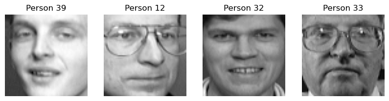

Now that we have our data loaded in, let's split it into training and testing sets.

from sklearn.model_selection import train_test_split

# Split the data into training and testing sets
X_train, X_test, y_train, y_test = train_test_split(faces_X, faces_y, test_size=0.2, random_state=1)

We can now initialize our two and fit our two models. We will use 100 trees for both models and default parameters otherwise for both models, timing how long it takes to fit each model. Starting with initialization,

# Initialize the models
gbc = GradientBoostingClassifier(n_estimators=100, random_state=1)
rf = RandomForestClassifier(n_estimators=100, random_state=1)

Now, let's fit our models and time how long it takes to fit each model, starting with the gradient boosting model.

%%timeit
gbc.fit(X_train, y_train)
>>> 10min 36s ± 1.89 s per loop (mean ± std. dev. of 7 runs, 1 loop each)

Now, let's fit our random forest model and time how long it takes to fit.

%%timeit
rf.fit(X_train, y_train)
>>> 1.36 s ± 4.24 ms per loop (mean ± std. dev. of 7 runs, 1 loop each)

As we can see, the random forest models took significantly less time to train than the gradient boosting model. It took 88 minutes and 12 seconds to fit the gradient boosted model, and 10.9 seconds to fit the random forest model. Now, just because training the random forest took less time does not mean the random forest model is better than the gradient boosting model. So let's see how well each model performs on the test set. We have

gbc.score(X_test, y_test)
>>> 0.5375

rf.score(X_test, y_test)
>>> 0.9125

Now, this is interesting. The random forest model took significantly less time to train, and it performed better on the test set. This is not to say that gradient boosting is bad. In fact, gradient boosting is a very powerful technique. However, it is important to understand that gradient boosting is not always the best choice for classification tasks. In this case, random forests outperformed gradient boosting. In other cases (such as one the fashion mnist dataset), I have seen gradient boosting outperform random forests. Gradient boosting should simply be another tool in your toolbox that you can use when you need it!

Also, gradient boosting is pretty obsolete now. It was a great technique when it was first introduced, but now algorithms such as XGBoost and LightGMB are much better and faster than gradient boosting. I will write a blog post about XGBoost and LightGBM in the future.

Conclusion

In this article, we talked about the math behind gradient boosting and talked a bit about using AdaBoost for classification. We discussed the why boosting is a good idea, and compared gradient boosting and random forests in Python! I hope that through this article, you now understand gradient boosting especially because of its importance in laying the foundation for other boosting algorithms. If you want to see the code used in this article, you can find it on my Github. I hope you delve deeper into gradient boosting on your data science and machine learning journey!