Dylan Skinner Blog

"We learn the rope of life by untying its knots."

- Jean Toomer

Knot theory is a branch of topology that studies the properties of mathematical knots. In this blog post, we will briefly explore the basics of knot theory and define some common terms used in the field. This blog post is a high level introduction to knot theory that is meant to not only be accessible to a general audience, but also prepare you for more advanced topics in knot theory that I will cover in subsequent blog posts.

Introduction to Knot Theory

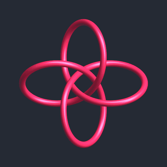
When a non-mathematician thinks of a knot, they typically think about taking a piece of string and tying the two ends together in some specific way. In mathematics, knots are thought of differently. Instead of taking a piece of string and tying the two ends together, a mathematical knot can be thought of by taking the two ends of a necklace, tying a knot in the middle of the necklace, and then clasping the two ends together. This results in a knotted loop where the only way to untangle the knot in the middle of the necklace is to cut the necklace and remove the knot. Put another way, a knot is a knotted loop of string except that we think of the string as having no thickness, and its cross-section being a single point [1]. Similarly, a link is a collection of multiple knots linked together.

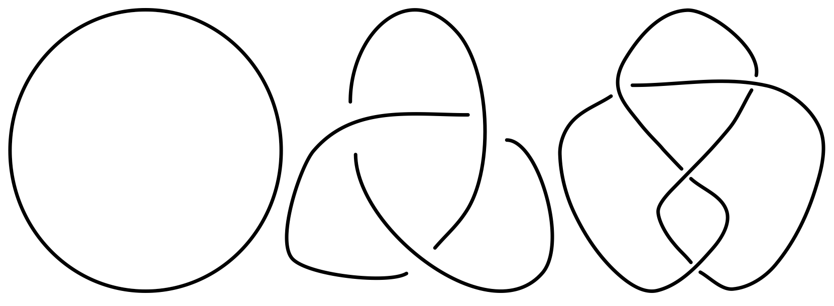
An important idea in knot theory is that there is no distinction between any particular configuration of a knot. In other words, if you take a knot and deform it in some way without passing it through itself or by cutting the string, the resulting knot is thought of as being the same as the original one. But, one problem arises from this idea. How can we tell when two different-looking knots are equivalent?

Before looking at the mathematical equivalence of knots, it is important to understand a few key terms. The first is projection. Knots live in three-dimensional space. However, it is often convenient to describe them using two-dimensional pictures. These two-dimensional pictures are obtained by projecting the three-dimensional knot onto a two-dimensional plane. If you were to take two 'different' projections of the same knot to a plane and create a model of one of those projections out of string, you should be able to rearrange the string into the second projection without cutting the string. This idea of rearranging the string in 3-dimensional space is something knot theorists call an ambient isotopy. Ambient refers to the fact that the string is being deformed in three-dimensional space, and isotopy the deformation of the string. When deforming a knot projection, knot theorists use the term planar isotopy, with planar referring to the fact that the knot is only being deformed within the projection plane.

This idea of isotopy is important in determining the equivalence of knots. Although two knots are considered equivalent if you can change one knot into the other by stretching it and moving it around without tearing it or causing the knot to intersect with itself, it is not immediately clear how this idea of 3-dimensional equivalence translates to 2-dimensional projections of the knot. In fact, it is a theorem that two knots are equivalent if and only if the projection of one knot can be transformed into that of another knot through a finite sequence of Reidemeister moves, as defined in Reidemeister's theorem below.

Reidemeister's Theorem

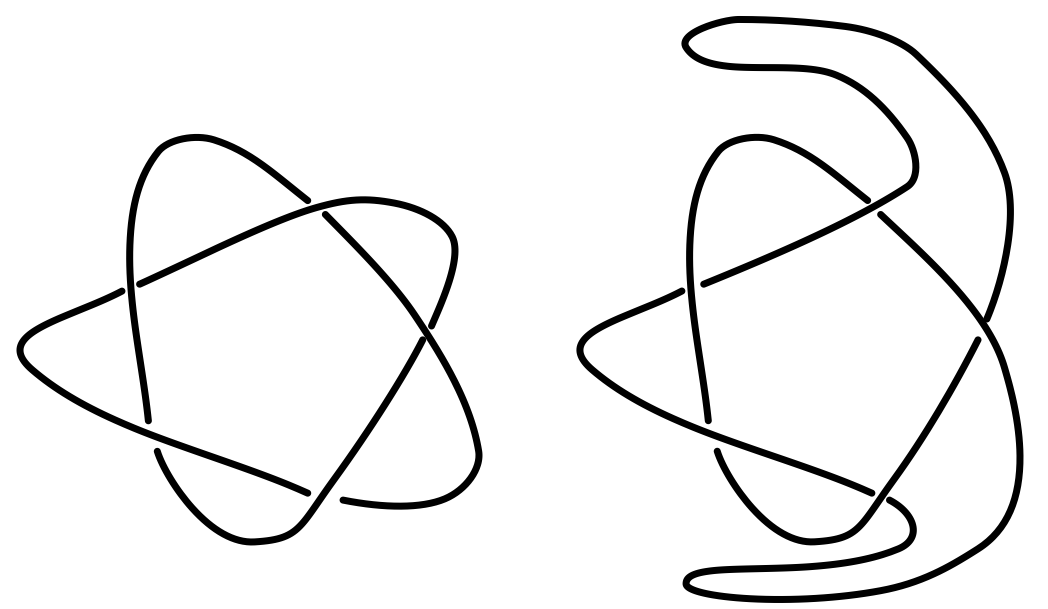
Reidemeister's theorem states that two links are ambient isotopic if and only if their diagrams can be joined by a sequence consisting of planar isotopies and the following three Reidemeister moves (see Figure 3):

• Move I: Twist and untwist in either direction.
• Move II: Move one strand over another.
• Move III: Move a strand completely over or under a crossing.

For more information about this theorem, you can check out chapter 1.4 in [1].

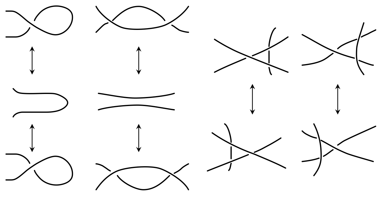
Reidemeister moves represent three different changes that can be made to a knot projection which do not change the equivalence class of the knot itself. The first Reidemeister move (or Reidemeister move I) is done by twisting or untwisting the knot. This twist will create another crossing but does not change the knot. Reidemeister move II is done by pushing one strand above or below another strand. This push can be used to create two new crossings, or remove two existing crossings. Reidemeister move III involves sliding a strand from one side of a crossing to the other side of that same crossing. This will not change the number of crossings present.

These Reidemeister moves are often referred to as twisting (move I), poking (move II), or sliding (move III) a knot, and represent the only three ways to change the projection of a knot, together with planar isotopy, without changing the knot itself. These moves are named after Kurt Reidemeister, a German mathematician, who proved in 1926 that if there are two distinct projections of the same knot, one can be transformed into the other by a sequence of these three moves and planar isotopy.

Conclusion

In this blog post, we have introduced the basics of knot theory and defined some common terms used in the field. We have also discussed Reidemeister's theorem, which states that two links are ambient isotopic if and only if their diagrams can be joined by a sequence consisting of planar isotopies and the three Reidemeister moves. In subsequent blog posts, we will explore more advanced topics in knot theory, including braids, surfaces, Markov's theorem, and slice surfaces.

Citations

[1] Collin C. Adams, The Knot Book. American Mathematical Society, 2004.