Dylan Skinner Blog

"Nobody can point to the fourth dimension, yet it is all around us."

- Rudy Rucker

Reinforcement learning is a type of machine learning that is concerned with how an agent should take actions in an environment in order to maximize some notion of cumulative reward. In this blog post, we will begin a brief introduction to reinforcement learning by talking about the Markov decision process (MDP).

What is Reinforcement Learning?

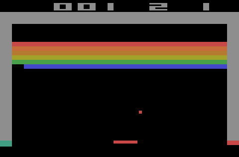
Reinforcement learning (RL) is a branch of machine learning that allows an agent to interact with an environment that it is placed in and to learn from the results of its interactions. When the agent is placed into an environment it is given a set of actions that it is allowed to take, which is how it interacts with the environment. The goal of reinforcement learning is to train the agent in such a way that it learns to select actions that yield optimal results given whatever situation it is in. As a simple example, consider the Atari game Breakout. The goal of the game is to break all the bricks in the level, which is done by using the paddle to hit a ball at the bricks. Tackling this problem using reinforcement learning, the agent controls the paddle and learns to move it in the most efficient way to break the bricks.

When an agent begins training, it is passed a starting state $s_{0}$ from the environment. The agent looks at this state, thinks about what it knows (which in the beginning is nothing), and selects an action $a_{0}$. This action is then sent back to the environment, analyzed, and assigned a reward $r_0$ based on the effect of the action on the environment. The environment then creates the next state $s_1$, and sends it and the reward $r_0$ back to the agent. This cyclical pattern occurs until the agent achieves the goal, fails, or some pre-determined number of time steps is reached. We can often model this situation as a Markov Decision Process (MDP)

The Markov Decision Process

An MDP is defined as $(S, A, R, \mathbb{P}, \gamma)$, where

• $S$ is the set of states,
• $A$ is the set of actions,
• $R$ is the distribution of rewards,
• $\mathbb{P}$ is the transition probabilities,
• $\gamma$ is the discount factor.

Reinforcement learning agents must learn decision making strategies not only in situations where actions create immediate rewards, but actions which impact rewards far into the future. In an MDP the current state $s_t$ tells us everything we need to know about the environment we are working in (this is called the Markov property). This is beneficial because there is no risk of filling up memory, but can be detrimental because all information about the past is essentially forgotten.

The goal of the agent utilizing the MDP is to pick an action to maximize the reward. To do this, the agent uses a policy $\pi$ which is a function that maps $S$ to $A$, represented as $\pi: S \to A$ (in some cases it is more useful to think of $A$ as a probability distribution across all actions, conditioned on the current state $s_t$). This function will pick an action based on the state the agent is in. Our hope is to find the best policy $\pi^{*}$ that will maximize the cumulative possible reward for the agent $\sum_{t=0}^{T}\gamma^{t}r_{t}$ (here the discount factor $\gamma$ is included so future rewards are not considered as heavily as current rewards). But this is a difficult task.

Through the work of researchers many different algorithms—both classical and ones that rely on deep learning— have been created to aid in finding $\pi^{*}$ in the most efficient way possible.

The Bellman Equation

In addition to the MDP, the Bellman Optimiality Principle is another key concept in reinforcement learning. Essentially, the Bellman optimality principle states that an optimal policy has the property that whatever the initial state and initial decision are, the remaining decisions must constitute an optimal policy with regard to the state resulting from the first decision. Meaning, for example, if the shortest path between Salt Lake City, UT and San Francisco, CA is through Elko, NV, then the shortest path between Elko and San Francisco must be through the shortest path between Salt Lake City and San Francisco. This principle is used to derive the Bellman equation, which is typically represented as: $$V(s) = \text{max}_a\left(R(s,a) + \gamma V(s')\right),$$ where

• $V(s)$ represents the 'value' of being in our current state,
• $R(s,a)$ is the reward we will get for taking action $a$ and being in state $s$,
• $\gamma$ is the discount factor, and
• V(s') represents the the value of being in the next state $s'$.

The $\text{max}_a$ tells us that the value of our current state is ultimately determined by the action that will yield the highest combination of immediate reward and future value. Note: that does not necessarily mean that the action with the highest immediate reward is the best action to take, but instead some combination of immediate reward and future value. Now, because there are typically multiple next states, the above equation is modified to $$V(s) = \text{max}_a\left(R(s,a) + \gamma \sum_{s'}p(s', a, s)V(s')\right)$$ This modification tells us that when figuring out the value of our current state, we must consider the value of all possible next states, and the probability of transitioning to those gates given our current state and action.

To calculate $V(s)$, we use dynamic programming to recursively calculate the value of each state. These results are often stored in a table for easy lookup. If using the Bellman equation, we can let our agent run through the environment and update the value of each state as it goes. Our hope is that eventually the value of each state will converge to the true value of the state, and we can use this information to determine the best action to take in each state. (This is often called value iteration.)

MDP vs. Bellman

When people talk about reinforcement learning, they will often mention the MDP and/or the Bellman equation and optimality principle. So, let's compare them real quick.

With the MDP, we have a memory benefit by not keeping track of all the previous states, but that can sometimes pose a problem because we lose all information about the past. The Bellman equation, on the other hand, allows us to know the value of each state, which is useful for determining the best action to take given whatever state we are in. However, not only can the Bellman equation be computationally expensive, but it also requires us to know the transition probabilities, which might not be known. Additionally, it is sometimes bold to assume that the state space is finite or can be discretized in a way that can be represented in a table.

Conclusion

In this blog post, we discussed the basics of the Markov decision process and the Bellman optimality principle and Bellman equation. These are fundamental concepts in reinforcement learning, and understanding them is crucial to understanding how reinforcement learning works. In future blog posts, we will discuss more advanced concepts in reinforcement learning, such as one of the optimal ways to calculate $\pi^*$.