Dylan Skinner Blog

"The biggest obstacle to creativity is breaking through the barrier of disbelief."

- Rodney Mullen

Proximal policy optimization (PPO) is a deep reinforcement learning (rl) algorithm that is quite good. In this blog post, we will dive into PPO, specifically breaking down the cost function (which is rather hairy).

What is PPO?

If you recall from my previous blog post on the Markov Decision Process, we discussed how an agent interacts with an environment. We also discussed that one of the most active fields of research in reinforcement learning is how to train an agent to make the best decisions possible; how to find $\pi^*$. PPO is one of the many algorithms that has been developed to help us find $\pi^*$, and it is currently the state-of-the-art!

PPO is a policy-based algorithm, meaning that it learns a policy $\pi$ that maps states to actions. The policy is learned by interacting with the environment and updating the policy based on the rewards received.

Additionally, PPO seeks to strike a balance between ease of implementation, sample complexity, and ease of tuning; all of which posed challenges to earlier algorithms. PPO does this by trying to compute an update at each step that both minimizes the cost function and only slightly deviates from the previous policy. This ensures that the agent does not take too big of steps and goes off track, but does not take steps that are too small which may lead to the agent going nowhere.

The Loss Function

In order for this to work, the algorithm utilizes two separate policy neural networks—the current policy $ \pi_{\theta}(a_{t}|s_{t})$, and the older policy $\pi_{\theta_{k}}(a_{t}|s_{t})$—and a rather unique objective function: $$L^{CLIP}(\theta) = \widehat{E}_{t}\Bigl[\text{min}\bigl( r_{t}(\theta)\widehat{A}_{t}, \text{clip}(r_{t}(\theta), 1 - \varepsilon, 1+\varepsilon)\widehat{A}_{t}\bigr) \Bigr],$$

where

• $\theta$ is the policy parameter,
• $\widehat{E}_{t}$ is the expected value (calculated by taking the average over a sequence of actions),
• $r_{t}(\theta)$ is the probability ratio, or the ratio of the current policy over the older policy, $\frac{\pi_{\theta}(a_{t}|s_{t})}{\pi_{\theta_{k}}(a_{t}|s_{t})}$. If $r_t(\theta) > 1$, it indicates that the new policy has a higher probability of selecting $a_t$ than the old policy. If it is less than 1, the new policy has a lower probability,
• $\widehat{A}_{t}$ is the estimated advantage at time step $t$, calculated as $\hat{A_{t}} = R_{t} - V(s_{t})$, where $R_{t}$ is the reward from the most recent action, and $V(s_{t})$ is the estimate of return starting from current state $s_t$, and
• $\varepsilon$ is a hyperparameter setting the size of the epsilon-neighborhood for step size.

One thing that makes this loss function interesting are the components inside of the minimization function. The first part, $r_{t}(\theta)\hat{A_{t}}$, is simply the probability ratio times the advantage. This is done to determine how much to update the policy for a specific action in a specific state as it quantifies the advantage of the action $a_t$ taken in state $s_t$ and its relative likelihood under the new and old policies. The second part, $clip(r_{t}(\theta), 1-\epsilon, 1+\epsilon)\hat{A_{t}}$, is a little bit different. If our new policy has a much higher probability of selecting $a_t$ than our old policy, then $r_t(\theta) \gg 1$. Similarly, if our new policy has a much lower probability of selecting $a_t$ than our old policy, we have $r_t(\theta) \ll 1$. This can be an issue because it can cause our algorithm to take a step too far in the wrong direction, potentially ruining its learning. The $\text{clip}$ function ensures all of our steps stay in a specified range. More specifically, if $r_t(\theta) < 1 - \epsilon$ or $r_t(\theta) > 1 + \epsilon$, the new value of $r_t(\theta)$ becomes $1 - \epsilon$ or $1 + \epsilon$, respectively.

Once $r_t(\theta)$ and $clip(r_t(\theta), 1-\epsilon, 1+\epsilon)$ are calculated, $L^{CLIP}$ selects the minimum of the two, and then finds the expected value of that result, thus allowing us to find the optimal step size.

The Algorithm

Let's now discuss how PPO works. The algorithm is quite simple, and can be broken down into the following steps:

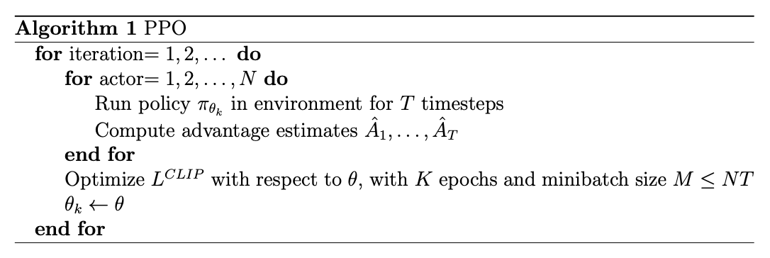
When the PPO runs, it starts off by running the old policy $\pi_{\theta_{k}}$, $N$ times for $T$ time steps. For each $n \in N$ iterations, the advantage $\hat{A_{t}}$ is calculated for each $t \in T$. Once the $N$ iterations are over, $L^{CLIP}$ is optimized with respect to $\theta$, and then $\pi_{\theta_{k}} \leftarrow \pi_{\theta}$.

In addition to these two policy networks, PPO also utilizes a value network. The value network is another neural network model used to estimate the expected cumulative reward (value) associated with a given state. It is used to assess the quality of states and provide feedback for policy improvement. There is only one of this network--not two networks like with the policy network.

Coding PPO

One of the best ways to understand an algorithm is to code it. Below is a simple implementation of the above algorithm using Pytorch (with the above loss function).

def learn_ppo(optim, policy, value, memory_dataloader, epsilon, policy_epochs):
    """Implement PPO policy and value network updates. Iterate over your entire 
       memory the number of times indicated by policy_epochs (policy_epochs = 5).    
  
      Args:
          optim (Adam): value and policy optimizer
          policy (PolicyNetwork): Policy Network
            policy_network = PolicyNetwork(state_size, action_size).cuda()
          value (ValueNetwork): Value Network
            value_network = ValueNetwork(state_size).cuda()
          memory_dataloader (DataLoader): dataloader with (state, action, action_dist, return) tensors
          epsilon (float): trust region
          policy_epochs (int): number of times to iterate over all memory
    """
    # Go through all epochs
    for epoch in range(policy_epochs):
      for batch in memory_dataloader:
        optim.zero_grad()
        
        # Get the all variables from memory (by batch)
        state, action, action_dist, return_v = batch

        # Do state.stack because we have a list of tensors, and we need a tensor of stuff.
        state = torch.stack(state, dim=1)      
  
        state_t       = state.type(torch.FloatTensor).cuda()
        action_t      = action.type(torch.LongTensor).cuda()
        action_dist_t = action_dist.type(torch.FloatTensor).cuda()
        return_v_t    = return_v.type(torch.FloatTensor).cuda()
  
        # Calculate advantage Â
        advantage = (return_v_t - value(state_t).cuda()).detach()
  
        # Calculate value loss
        value_loss = F.mse_loss(return_v_t, value(state_t).squeeze())
  
        # Calculate π(s,a)
        policy_norm       = action_dist_t.squeeze(1)
        action_onehot     = F.one_hot(action_t, 13).bool()
        taken_policy_norm = policy_norm[action_onehot]
        
        #Calculate π'(s,a)
        policy_prime       = policy(state_t)
        taken_policy_prime = policy_prime[action_onehot]
        
        #Calculate the ratio between π'(s,a)/π(s,a)
        prim_div_norm = taken_policy_prime / taken_policy_norm
  
        # Clipping π'(s,a)/π(s,a)
        clip = torch.clip(prim_div_norm, 1-epsilon, 1+epsilon)
        
        # Left part of the policy loss (π'(s,a)/π(s,a))*Â
        left_part = prim_div_norm * advantage

        # Right part of the policy loss clip*Â
        right_part = clip * advantage
  
        # Calculating policy loss
        policy_loss = torch.mean(torch.min(left_part, right_part))
  
        # Total loss
        total_loss = value_loss - policy_loss
        
        total_loss.backward()
        optim.step()

(To see a more complete implementation, check out my Github where I have implemented PPO to solve a 4D topology problem.)

Conclusion

In this blog post, we discussed the PPO algorithm and its loss function. We also discussed how to implement PPO in Pytorch. PPO is a powerful algorithm that has been used to solve a variety of problems, from playing video games to solving 4D topology problems! I encourage you to try implementing PPO in your own projects, and see how it can help you solve your problems. (I also invite you to check out the original PPO paper to learn more about the weeds of this algorithm.)