Dylan Skinner Blog

"If you optimize everything, you will always be unhappy."

- Donald Knuth

Behind important things like machine learning, finance, and operations research lies an important concept: optimization. Optimization is the process of finding the best solution to a problem from all possible solutions. In this blog post, we will discuss the basics of unconstrained optimization, a fundamental concept in optimization theory. We will specifically discuss a few necessary and sufficient conditions for optimality, and consider a few examples.

Some Important Definitions

Throughout this blog post, we will be working with a function $f: \Omega \rightarrow \mathbb{R}$, where $\Omega\in\mathbb{R}^n$ is an open set.

It is first important to define what it means for a value to be a minimizer. If we have our function $f$ as defined above, then we say a point $\textbf{x}^*\in\Omega$ is a minimizer of $f$ if $f(\textbf{x}^*) \leq f(\textbf{x})$ for all $\textbf{x}\in\Omega$. In this case, we call $f(\textbf{x}^*)$ the minimum value of $f$. We currently make no claims about either the uniqueness of the minimizer nor claim is is a global minimizer (but we will discuss this later). In this current set up, if there are no other constraints on the set of possible minimizers, then we say we are working with unconstrained optimization.

As mentioned above, it is very possible to have multiple minimizers of a function. It is typical to denote the set of all minimizers of $f$ as $$\text{argmin}_{\textbf{x}\in\Omega} \;f(\textbf{x}) = \{\textbf{x}\in\Omega \;|\; f(\textbf{x})\,\leq\, f(\textbf{y})\quad \forall\textbf{y}\in\Omega \}.$$ Of course, if this is a set with one element, then we say the minimizer is unique. It should also be mentioned that, by definition, this set will contain only minimizers that yield the global minimum value.

Necessary and Sufficient Conditions for Optimality

With these basic definitions and ideas under our belt, we can now discuss some necessary and sufficient conditions for optimality. We begin with the first order necessary condition for optimality.

First-Order Necessary Condition (FONC)

If we have our function $f$ as defined above with the additional condition that $f$ is differentiable, then if we know $\textbf{x}^*$ is a local minimizer of $f$, then $Df(\textbf{x}^*) = \mathbf{0}^T$.

To see this, let's suppose that we have a point $\textbf{x}^*$ that is a local minimizer of $f$, but $Df(\textbf{x}^*) \neq \mathbf{0}^T$. If this is true, then we can define a unit vector $\textbf{q} = -\frac{Df(\textbf{x}^*)^T}{\lVert Df(\textbf{x}^*)^T}$. This tells us that $Df(\textbf{x}^*)\textbf{q} = -\lVert Df(\textbf{x}^*)\rVert$. So, by the non-negative property of norms, we have that $Df(\textbf{x}^*)\textbf{q} = -\lVert Df(\textbf{x}^*)\rVert < 0$. Since $\textbf{x}^*$ is a local minimizer, this means that we can find a point $\textbf{x}^* + \alpha\textbf{q}$ such that $f(\textbf{x}^* + \alpha\textbf{q}) < f(\textbf{x}^*)$. By definition of the derivative, we have $$\begin{aligned} \frac{|f(\textbf{x}^* + t\textbf{q}) - f(\textbf{x}^*) - tDf(\textbf{x}^*)\textbf{q}|}{\lVert t\textbf{q}\rVert} &= \frac{f(\textbf{x}^* + t\textbf{q}) - f(\textbf{x}^*) + t\lVert Df(\textbf{x}^*)\rVert}{|t|} \\ &= \frac{f(\textbf{x}^* + t\textbf{q}) - f(\textbf{x}^*) + t\lVert Df(\textbf{x}^*)\rVert}{t} \\ &= \frac{f(\textbf{x}^* + t\textbf{q}) - f(\textbf{x}^*)}{t} + \lVert Df(\textbf{x}^*)\rVert \geq \lVert Df(\textbf{x}^*) \rVert. \end{aligned}$$ This implies that $$\frac{f(\textbf{x}^* + t\textbf{q}) - f(\textbf{x}^*)}{t} \geq 0$$ However, by definition of the derivative, we have $$\frac{|f(\textbf{x}^* + t\textbf{q}) - f(\textbf{x}^*) - tDf(\textbf{x}^*)\textbf{q}|}{\lVert t\textbf{q}\rVert} = 0,$$ so we conclude with $0\geq 0$, which is a contradiction. Thus, we must have that $Df(\textbf{x}^*) = \mathbf{0}^T$.

With this in mind, we know that a point can only be a local minimizer if the derivative of the function at that point is zero. That is not to say that every point where the derivative is zero is a local minimizer, but a point is certainly not a local minimizer if the derivative is not zero.

(While the FONC has a very simple statement, it should be noted that it is not always easy to verify $Df(\textbf{x}) = 0$. This is important to find keep in mind.)

Second-Order Necessary Condition (SONC)

In addition to the first-order necessary condition, we can also consider the second-order necessary condition. This condition is a little more involved, but it is still important to consider.

For second-order conditions, we utilize what is called the Hessian or second-derivative matrix. The Hessian of a function $f$ is defined very generally as $$ \textbf{H}_f = D^2f(\textbf{x}) = \begin{bmatrix} \frac{\partial^2 f}{\partial x_1^2} & \frac{\partial^2 f}{\partial x_1\partial x_2} & \cdots & \frac{\partial^2 f}{\partial x_1\partial x_n} \\ \frac{\partial^2 f}{\partial x_2\partial x_1} & \frac{\partial^2 f}{\partial x_2^2} & \cdots & \frac{\partial^2 f}{\partial x_2\partial x_n} \\ \vdots & \vdots & \ddots & \vdots \\ \frac{\partial^2 f}{\partial x_n\partial x_1} & \frac{\partial^2 f}{\partial x_n\partial x_2} & \cdots & \frac{\partial^2 f}{\partial x_n^2} \end{bmatrix}.$$ With this in mind, we define the SONC to be if $\textbf{x}^*$ is a local minimizer of $f$, then the Hessian $D^2f(\textbf{x}^*)$ is positive semidefinite (also denoted $D^2f(\textbf{x}^*) \geq 0$). Now, the term positive semidefinite might be new to you, but it simply means that all the eigenvalues of the matrix are nonnegative ($\lambda \geq 0$ $\forall\lambda\in\sigma(D^2f(\textbf{x}^*))$).

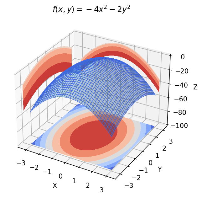
Rather than dive into the proof (which is not very exciting to me), let's instead consider an example. Consider the function $f(x) = -4x^2 - 2y^2$. The first derivative of the function is defined as $Df(x, y) = \begin{bmatrix} -8x, & -4y \end{bmatrix}$. We can easily see that the only place where $Df(x,y) = 0$ is at the origin $(0,0)$. So the origin is the only point that could be a local minimizer (though not guaranteed). The second derivative of the function is defined as $$D^2f(x, y) = \begin{bmatrix} -8 & 0 \\ 0 & -4 \end{bmatrix}$$. In this case, the eigenvalues of the Hessian are $-8$ and $-4$, which are both negative. Thus, our Hessian matrix is negative definite everywhere, so we can conclude the origin is not a local minimizer. This is of course a toy example and can be easily verified by graphing the function (see below). But the idea is important.

Second-Order Sufficient Condition (SOSC)

Now, up to this point, we have only discussed necessary conditions for optimality. That is, we have only discussed conditions that, if a point $\textbf{x}^*$ is a local minimizer, then those conditions are true. We will now discuss a sufficient conditions for optimality, namely the second-order sufficient condition.

We define the second-order sufficient condition (SOSC) to be if $\textbf{x}^*\in\Omega$ is a point such that $Df(\textbf{x}^*) = \mathbf{0}^T$ and $D^2f(\textbf{x}^*)$ is positive definite (denoted $D^2f(\textbf{x}^*) > 0$), then $\textbf{x}^*$ is a local minimizer of $f$. (This idea of positive definite is similar to positive semidefinite, but all the eigenvalues are positive.)

We should note that this sufficiency condition does not say anything about the point $\textbf{x}^*$ being a global minimizer. It only says that if the conditions are met, then $\textbf{x}^*$ is a local minimizer.

Let's see SOSC in action with a fun example.

The Rosenbrock Function

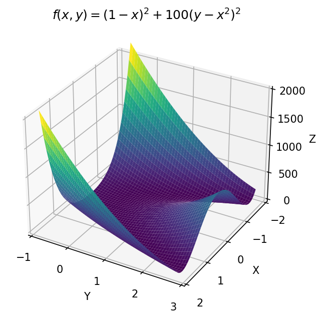
We will show the power of the SOSC with the Rosenbrock function. The Rosenbrock function is often used as a test function for optimization algorithms because of how difficult it is to find the simple minimizer numerically. This difficulty arises from the fact that the function has a very flat valley that the optimizer must traverse to find the minimum. We define the Rosenbrock function to be $f(x,y) = (1-x)^2 + 100(y-x^2)^2$. Here is a plot to visualize it.

Let's do some math to get the local minimizer! Recall that SOSC tells us that if $Df(\textbf{x}^*) = \mathbf{0}^T$ and $D^2f(\textbf{x}^*) > 0$, then $\textbf{x}^*$ is a local minimizer. So, let's start by getting some derivatives. The first derivative of the Rosenbrock function (and setting it equal to zero) is $$\begin{aligned} Df(x, y) &= \begin{bmatrix} -2(1-x) - 400x(y-x^2), & 200(y-x^2) \end{bmatrix} \\ &= \begin{bmatrix} -2 + 2x -400xy + 400x^3, & 200y - 200x^2 \end{bmatrix} = \begin{bmatrix} 0, & 0 \end{bmatrix}. \end{aligned}$$ Solving the second entry of the vector, we get $y = x^2$. Plugging this into the first entry, we get $$-2(1-x) - 400x({\color{red}x^2}-x^2) = 0 \implies -2(1-x) - {\color{red}0} = 0 \implies x = 1.$$ Since $y = x^2$ and $x=1$, we have $y=1$. Thus, our candidate point (or critical point) is $(1,1)$. Now, let's find the Hessian of the Rosenbrock function. The Hessian is $$D^2f(x, y) = \begin{bmatrix} 2 - 400y + 1200x^2 & -400x \\ -400x & 200 \end{bmatrix}.$$ Evaluating our Hessian at $(1,1)$, we get $$D^2f(1, 1) = \begin{bmatrix} 2 - 400{\color{red}(1)} +1200{\color{red}(1)}^2 & -400{\color{red}(1)} \\ -400{\color{red}(1)} & 200 \end{bmatrix} = \begin{bmatrix} 802 & -400 \\ -400 & 200 \end{bmatrix}.$$ We can now check if $D^2f(1,1)$ is positive definite by looking at the eignevalues. Using a computational solver, we get $\lambda = 501 \pm \sqrt{250601} \approx \{1001.6, 0.399 \}$. Since both of these are positive always, $D^2f(1,1)$ is positive definite. Thus, by SOSC, we have that $(1,1)$ is a local minimizer of the Rosenbrock function.

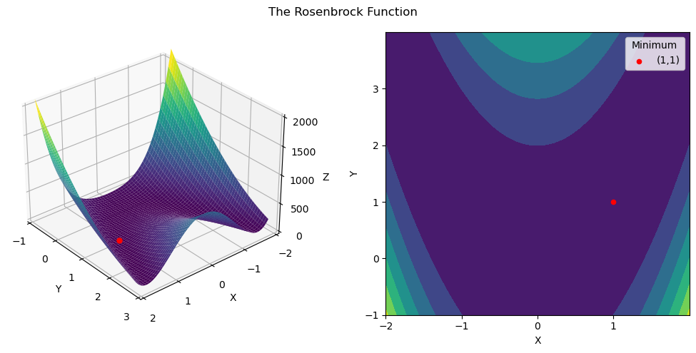
This is a very powerful result! Looking at the graph of the Rosenbrock function, it is very difficult to see that $(1,1)$ is a minimizer. But, by using the SOSC, we can see that it is indeed a local minimizer.

Conclusion

Unconstrained optimization is a very important concept in optimization theory. In this blog post, we discussed some necessary and sufficient conditions for optimality. We discussed the first-order necessary condition (FONC), the second-order necessary condition (SONC), and the second-order sufficient condition (SOSC). We also considered the Rosenbrock function as an example of how to use these conditions. Unconstrained optimization plays a huge role in many complex fields and is even the backbone of tools like gradient descent. (If you want to see how I built the plots for this blog post, you can check them out here.)