Dylan Skinner Blog

"Braids, bouffants, and balayage. Everything a girl wants to hear"

- The Internet

Continuing on from my previous blog post, this blog post focuses on braids, Alexander's Theorem, and Markov's Theorem.

Introduction to Braids

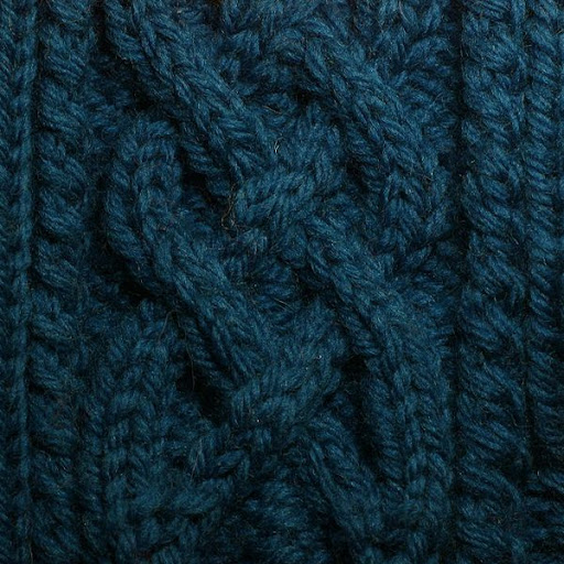
In knot theory, knots can be represented in many different ways besides using the planar projections described in my previous blog post. One of these ways is using braid closures. Braids are particularly helpful because every knot can be described as the closure of a braid. A braid is a set of $n$ strings that are attached to a horizontal bar at the top and the bottom and which travel monotonically downwards (see Figure 1). These strings can cross over or underneath each other, but they cannot loop back up. Another way of putting this is that each string can cross any horizontal plane only one time. We let $B_n$ denote the set of all braids with $n$ strands.

Similar to knots, there is a notion of equivalency for braids. In order to see that two braids are equivalent, we must be able to rearrange the strings of the braid without removing the strings from the top or bottom bar, and without allowing the strings to pass through each other or themselves.

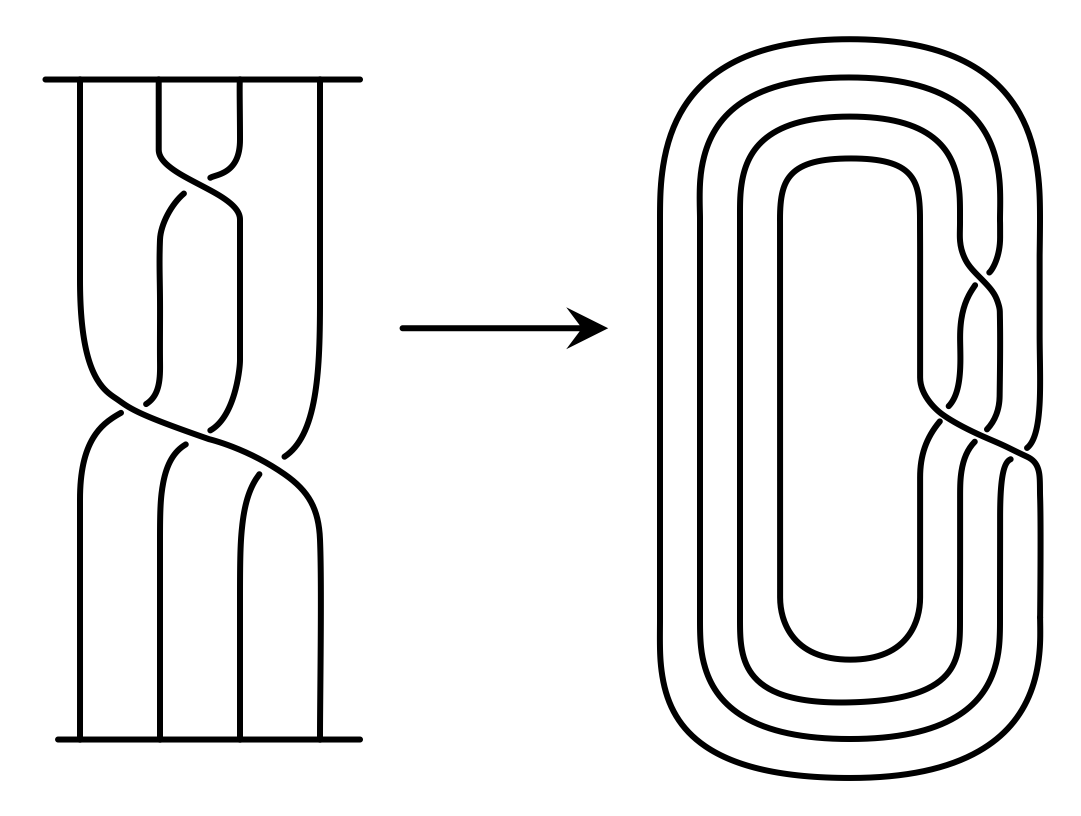
When we have a braid, we can turn that braid into a knot by connecting the top and bottom bars together. The resulting form is a knot or a link, and this is called the closure of the braid (see Figure 3).

As mentioned previously, one nice feature of braids is that every knot can be represented as the closure of a braid. This helpful fact was proven by J.W. Alexander in 1923 and is known as Alexander's Theorem.

Alexander's Theorem

Alexander's theorem states that every knot or link can be expressed as the closure of a braid. (See chapter 5.4 in [1] for more.)

Simple as this theorem may be, it is incredibly helpful for working with knots. Since every knot can be represented as a braid closure, we have another useful way of studying and classifying knots. In the same vein, one useful quantity to consider when thinking of knots as braid closures is the braid index.

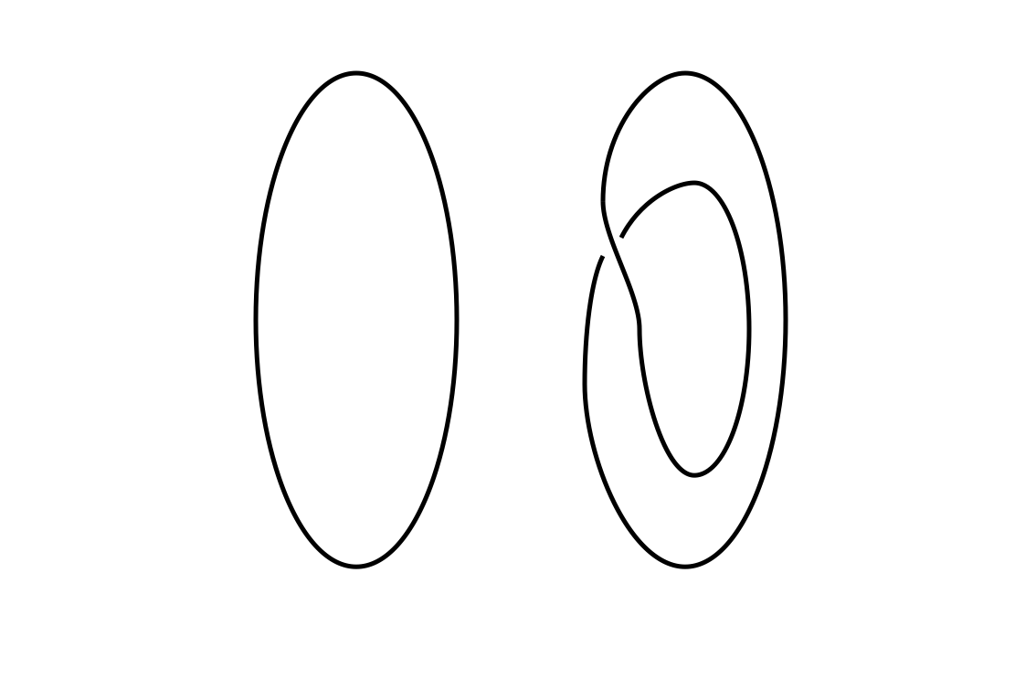
The braid index of a knot is defined to be the fewest number of strings in a braid whose closure is the knot of interest [1]. For example, the unknot (which is simply a circle) has a braid index of 1 since it can be expressed as the closure of a braid with a single strand (and no crossings).

While calculating the braid index seems simple, it can actually be quite tricky. If we represent a knot in braid form and then count the strings of the braid, it does not guarantee that we have achieved the least number of strings possible for that knot. Counting the strings of a braid representative can certainly give us an upper bound on the braid index, but finding the actual minimal braid index requires more work.

Braid Words

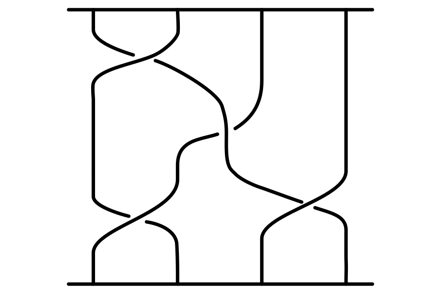
In order to fully describe a braid, we look first at its projection. Once we have the projection of the braid—and ensure that no two crossings occur at the same height—we describe the braid by listing the strings that cross over and under other strings as we move toward the bottom bar. We always label the crossings from left to right. When the first string crosses under the second string, we call this crossing a $\sigma_{1}$ crossing. On the other hand, if the first string crosses over the second string, we call this crossing a $\sigma_{1}^{-1}$ crossing. If the second string crosses under the third, it is a $\sigma_{2}$ crossing, and if the second string crosses over the third, it is a $\sigma_{2}^{-1}$ crossing. This pattern continues, with a crossing of the $j^{th}$ strand passing under the $(j+1)^{th}$ strand being labeled as $\sigma_j$, while $\sigma_j^{-1}$ denotes the $j^{th}$ strand passing over the $(j+1)^{th}$ strand. To describe a braid then we simply start at the top of the braid, and list off the crossings we encounter as we travel from top to bottom. We call the resulting sequence of crossings a braid word.

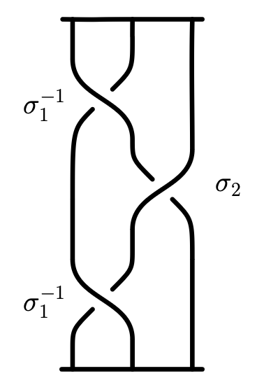
If we look at the braid in Figure 5, we can see that by listing the crossings from top to bottom, we obtain the braid word $\sigma_{1}^{-1}\sigma_{2}\sigma_{1}^{-1}$.

Along with giving a convenient way to describe the braid, there are other advantages to using braid representations of knots. One advantage is identifying which Reidemeister moves can be applied to simplify the braid. For example, if a braid word contains $\sigma_{k}\sigma_{k}^{-1}$, we know that the $k^{th}$ string goes under the ${(k+1)}^{th}$, and then immediately passes back underneath of it, returning to its original position. If we apply a simple Reidemester II move to this pair of crossings, the strings will straighten out and we are left with an equivalent braid (see Figure 6).

For a more complicated example, say we have the braid word $\sigma_{1}\sigma_{3}\sigma_{2}\sigma_{2}^{-1}\sigma_{3}^{-1}\sigma_{4}\sigma_{3}$. Through a series of Reidemester II moves, we can take this word and simplify it to $\sigma_{1}\sigma_{3}\sigma_{3}^{-1}\sigma_{4}\sigma_{3}$, and then further to $\sigma_{1}\sigma_{4}\sigma_{3}$. This leaves us with a much simpler braid word which represents a braid that is equivalent to the original braid.

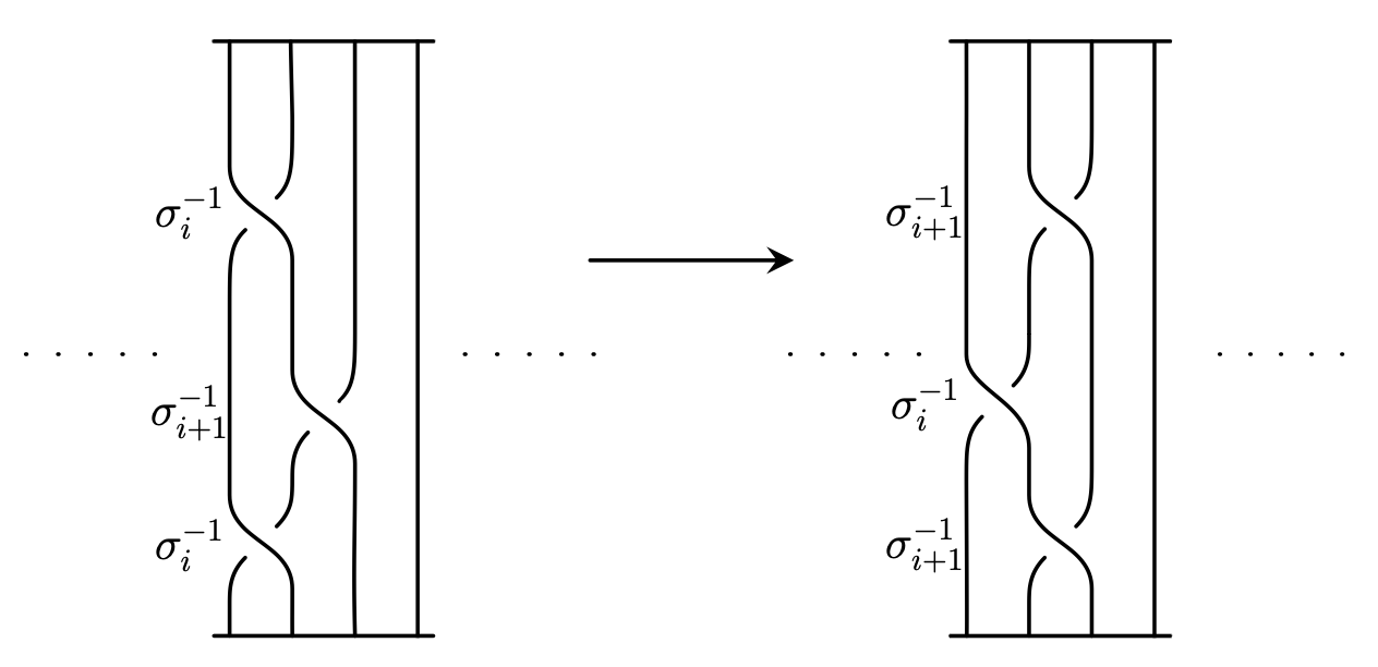
Another modification we can apply to braid projections is the Reidemeister III move. If we are given a braid projection and wish to move a strand over or under a crossing we are allowed to do this since a string does not need to be cut in the process. In general if you braid word contains $\sigma_{i}\sigma_{i+1}\sigma_{i}$, for $1 \leq i \leq n-2$, then it can be replaced using the substitution $\sigma_{i}\sigma_{i+1}\sigma_{i} = \sigma_{i+1}\sigma_{i}\sigma_{i+1}$ (see Figure 7, where the equivalent substitution $\sigma_{i}^{-1}\sigma_{i+1}^{-1}\sigma_{i}^{-1} = \sigma_{i+1}^{-1}\sigma_{i}^{-1}\sigma_{i+1}^{-1}$ is illustrated).

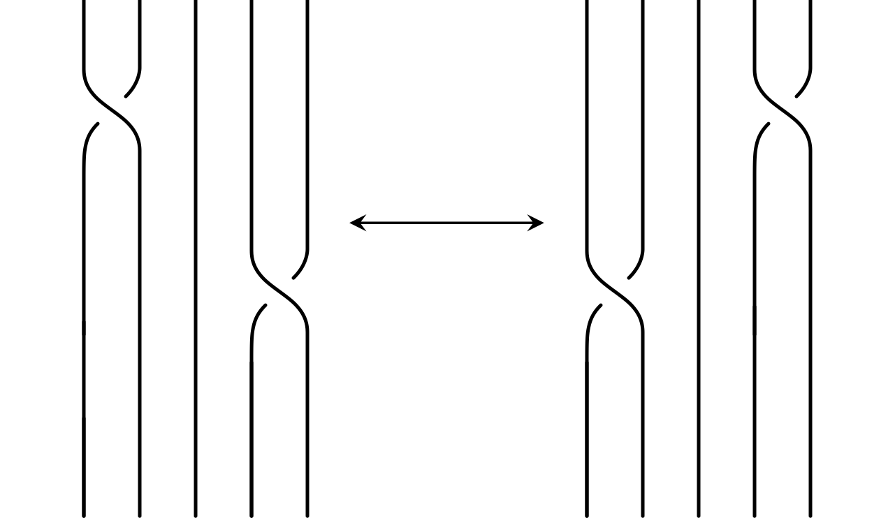
The final move that we can apply to braid projections is not a Reidemeister move; instead, it is a switch. If our braid word contains $\sigma_{i}\sigma_{j}$, where $|i-j| > 1$, then we can switch the order of $\sigma_{i}$ and $\sigma_{j}$. So $\sigma_{i}\sigma_{j}$ becomes $\sigma_{j}\sigma_{i}$ (see Figure 8).

Using these three moves allows us to determine when two braids $b_{1}$ and $b_{2}$ are equivalent. This ideas leads to another very important theorem for working with braids: Markov's theorem.

Markov's Theorem

Markov's theorem [2] states:

Given two braid words $\beta_{n}\in B_{n}$, $\beta'_{m}\in B_{m}$ with $n$ and $m$ strands respectively, their closures are equivalent links if and only if $\beta'_{m}$ can be obtained from $\beta_{n}$ by applying a sequence of the following operations:

1. conjugating $\beta_{n}$ in $B_{n}$;
2. replacing $\beta_{n}$ by $\beta_n\sigma_{n}^{\pm 1} \in B_{n+1}$;
3. the inverse of the previous operation (if $\beta_{n}=\beta_{n-1}\sigma_{n}^{\pm 1}$ with $\beta_{n-1} \in B_{n-1}$, replace $\beta_{n}$ with $\beta_{n-1}$).

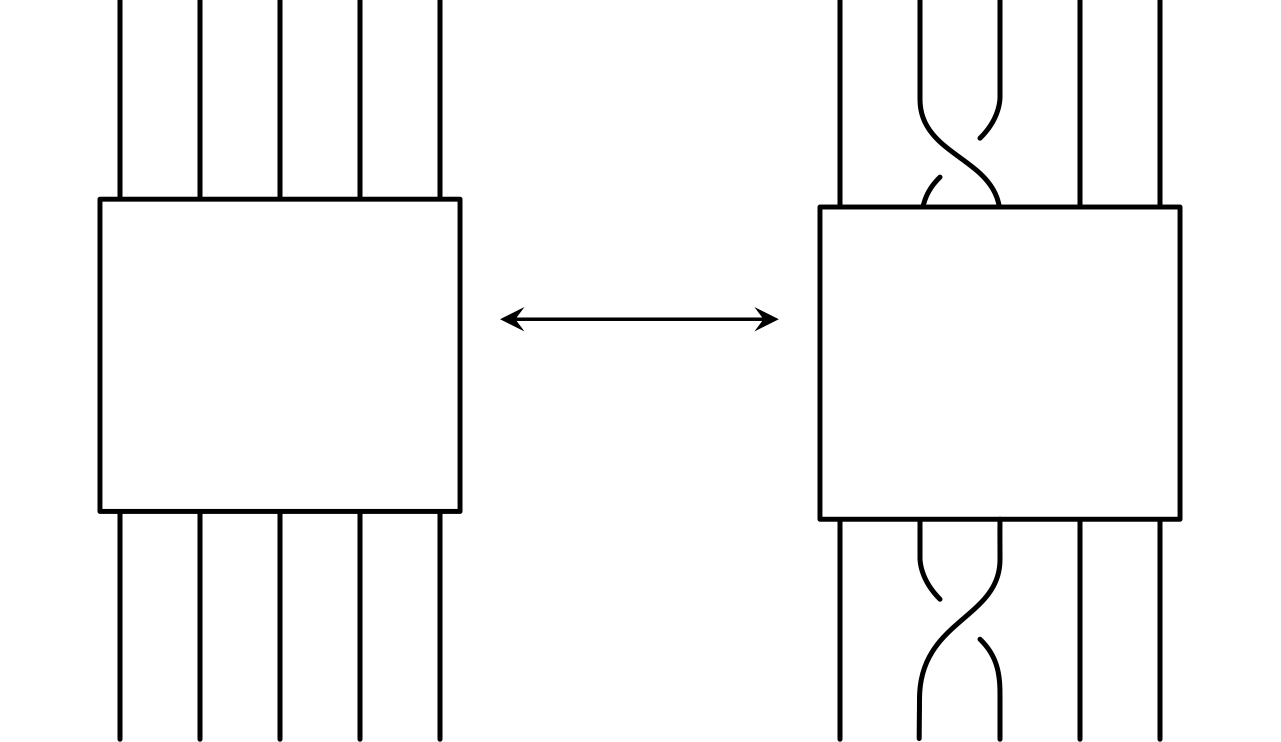
In Markov's theorem, we learn about two new moves that can be applied to braids to obtain different braids with equivalent closures. The first comes in part 1: conjugation. Conjugation is an operation applied to the braid word where the beginning of the word is multiplied by $\sigma_{j}$, and the end of the word by $\sigma_{j}^{-1}$, or vice-versa. In the closure we are only adding a Reidemeister II move, so we are not changing the resulting knot type (see Figure 9).

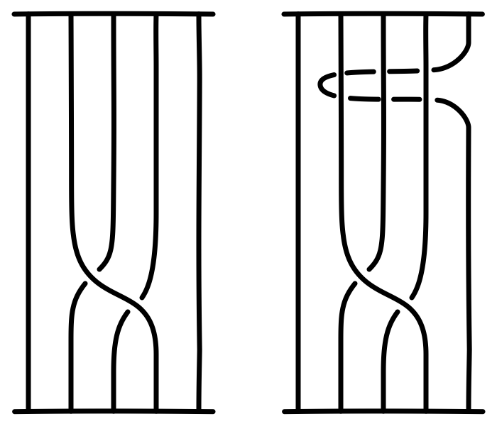
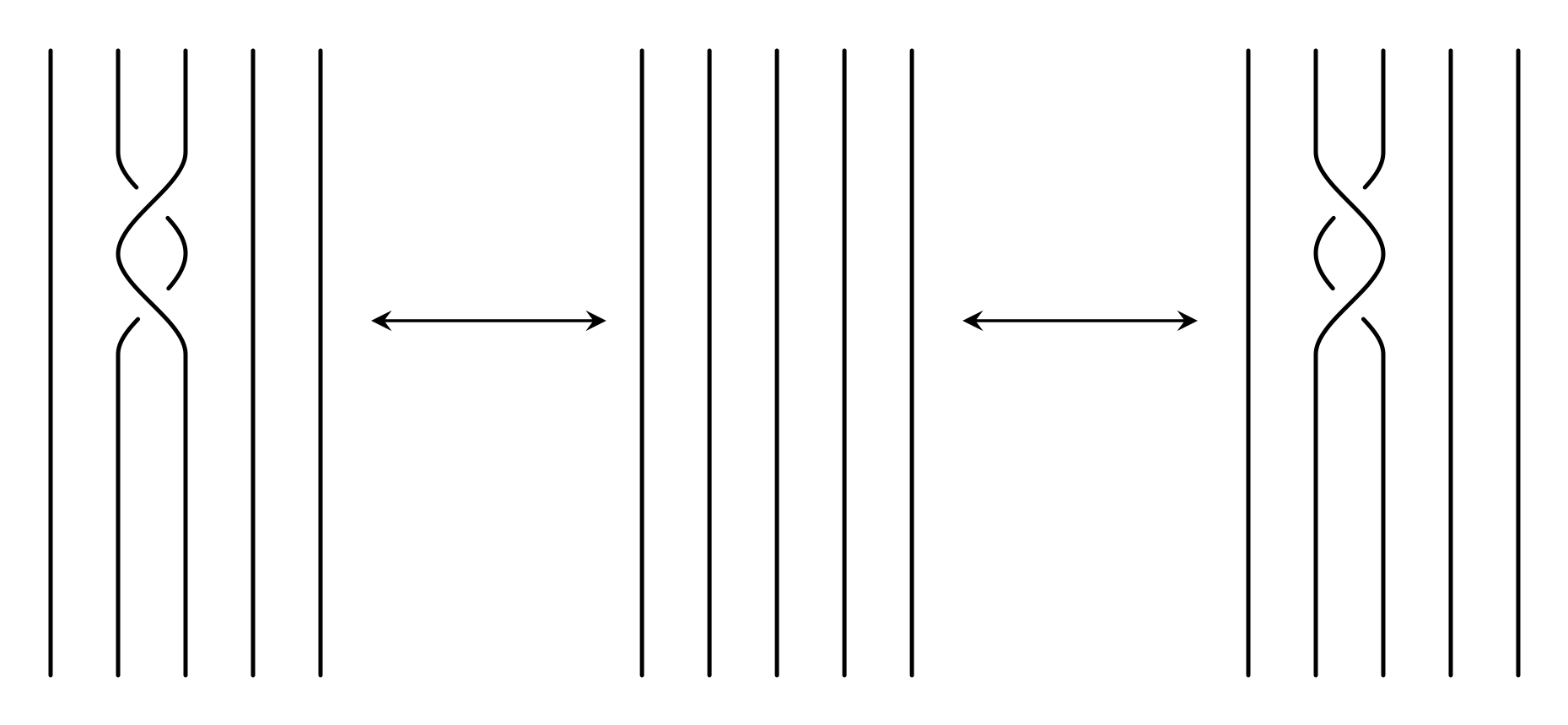
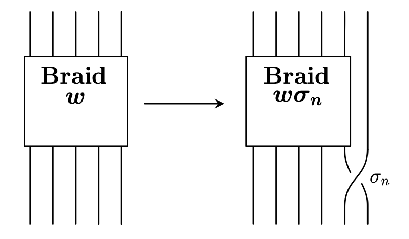
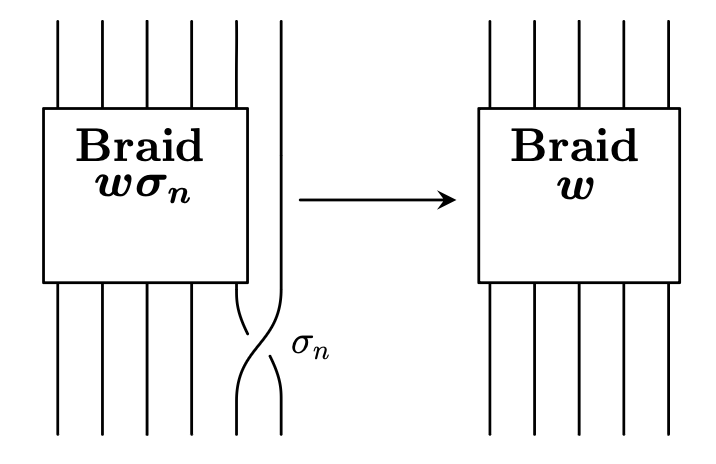
The second move comes in part 2: stabilization. Stabilization involves adding a new strand and a single crossing to a braid as illustrated in Figure 10. This is performed by taking the braid word $w$ that corresponds to an $n$-string braid, adding a strand to make it an $(n+1)$-string braid, and then adding $\sigma_{n}$ or $\sigma_{n}^{-1}$ to the beginning or end of the word $w$. Destabilization is the opposite of stabilization: simply remove a string and a crossing from a braid as shown in Figure 11 below.

Conclusion

In this blog post, we discussed the basics of braids and introduced Alexander's theorem, and Markov's Theorem. Alexander's theorem which states that every knot or link can be expressed as the closure of a braid, and Markov's theorem which states that two braids are equivalent if and only if their diagrams are similar through a sequence of conjugations, stabilizations, and destabilizations. This is a precursor for the next blog post which will be about slice surfaces.

Citations

[1] Collin C. Adams, The Knot Book. American Mathematical Society, 2004. ISBN: 978-0821836781.

[2] Joan S Birman. Braids, links, and mapping class groups. 82. Princeton University Press, 1974.