Dylan Skinner Blog

"All we're doing is going down hill."

- Dr. Ben Webb

Gradient descent is one of the key innovations that allows us to optimize functions. It is a simple algorithm with a simple goal: solving unconstrained optimization problems of the form $$\text{minimize} \;f: \mathbb{R}^n\to\mathbb{R}.$$

In a previous blog post we discuessed unconstrained optimization and some of the necessary and sufficient conditions for optimality. In this blog post, we will make the optimization a little more complicated by taking about gradient descent, Polyak's heavy ball method, and Nesterov's accelerated gradient descent method. Don't be afraid, though! In the words of one of my college professors, Dr. Ben Webb, "All we're doing is going down hill."

The Basics of Gradient Descent

If you can recall from your multivariate calculus class (and if you never took multivariate calculus, that's okay), the gradient $Df(\textbf{x})^{\intercal}$ of a function $f$ is a vector that points in the direction of the greatest increase of the function at a point $\textbf{x}$. This tells us that the negative gradient $-Df(\textbf{x})^{\intercal}$ points in the direction of the greatest decrease of the function at a point $\textbf{x}$. This idea of the negative gradient is exactly the intuition behind gradient descent.

So, we define the basic form of gradient descent to be $$\textbf{x}_{k+1} = \textbf{x}_k - \alpha Df(\textbf{x}_k)^{\intercal},$$ where $\textbf{x}_k$ is the current point, $\textbf{x}_{k+1}$ is the next point, and $\alpha$ is a step size (or learning rate) that we can adjust.

This is a very simply algorithm to code up with one simple implementation being as follows:

import numpy as np
import scipy.optimize as opt

# Define our gradient descent function
def gradient_descent(f, x0, lr=0.1, tol=1e-6, maxiter=10**5):
    # Get our initial guess
    x_vals = np.array([x0])
    x = x0
    
    # Iterate until we converge
    for i in tqdm(range(maxiter)):
        # Get the gradient
        grad = opt.approx_fprime(x, f, 1e-6)
        
        # Update our guess
        x = x - lr * grad
        x_vals = np.vstack((x_vals, x))
        
        # Check for convergence
        if np.linalg.norm(grad) < tol:
            break
    return x_vals, i

In this implementation, we use the approx_fprime function from the scipy.optimize package to approximate the gradient of the function $f$ at a point $\textbf{x}$. This could also be doing using something like jax or your favorite difference method for calculating derivatives.

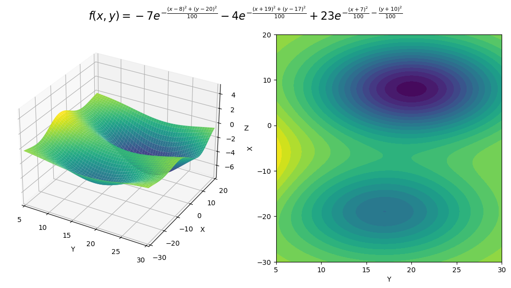
To visualize how this code works, consider the following function: $$f(x,y) = -7e^{-\frac{(x-8)^2 + (y-20)^2}{100}} - 4e^{-\frac{(x+19)^2 + (y-17)^2}{100}} + 23e^{-\frac{(x+7)^2}{100} - \frac{(y+10)^2}{100}}.$$ This function has two minima. A local minimum at the point $(-19, 17)$, and a global minimum at the point $(8, 20)$. We can visualize this function with the following plot.

To see how gradient descent works, we can start at a point $(x_0, y_0)$ (which we pick randomly), and then follow the recursive formula until a convergence criterion is met. In this case, we define the convergence criterion to be when the norm of the gradient is less than $10^{-8}$. We can visualize this process with the following gif.

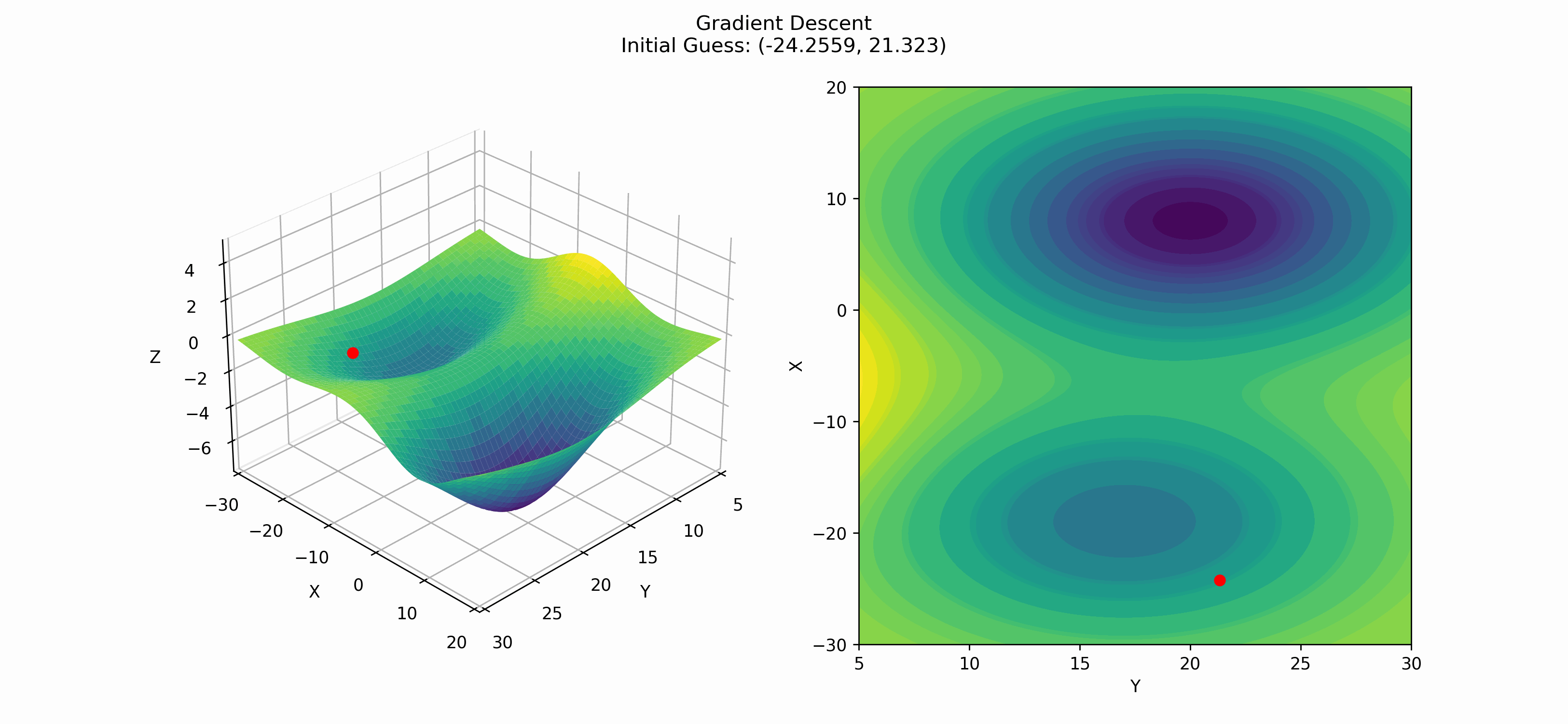
In this gif, we are able to see both a strength and a weakness of gradient descent. The strength is that gradient descent is able to go downhill towards a minimum. The weakness is it finds a local minimum rather than a global minimum. This is a common problem in optimization and does not have a one-size-fits-all answer. There have been some research into fixing this problem, which we will now talk about.

Polyak's Heavy Ball Method

As seen in the previous section about Gradient Descent, we find the next point in our optimization by taking a step in the direction of the negative gradient. This gives us a progression of points that should lead us to a minimum. We can use this information and a few ideas from physics to improve our optimization. One idea is to think of a ball rolling down a hill. If the ball is heavy, it will have more momentum and will be able to roll further down the hill. This ball will have a particular velocity that we can find by looking at the current and previous positions of the ball and how long the point update took. In the case of gradient descent, since the time it takes to get from one point to the next is simply one time step, we can create an auxiliary variable $\textbf{v}_k$ that represents the velocity of our point and is given by $$v_k = \textbf{x}_{k+1} - \textbf{x}_k.$$ Notice, we find the velocity is always one step behind the current point. This should make sense because it is impossible to tell the velocity of the ball at the current point if we're not sure where the ball will be next. This is the idea behind Polyak's Heavy Ball Method.

Differing from the basic gradient descent algorithm, Polyak's Heavy Ball Method is given by $$\textbf{x}_{k+1} = \textbf{x}_k - \alpha Df(\textbf{x}_k)^{\intercal} + \beta(\textbf{x}_k - \textbf{x}_{k-1}),$$ where $\beta$ is a momentum parameter that we can adjust. If $\beta = 0$, this is simply gradient descent. It is common to choose $\beta\in(0, 1)$.

There are two other ways to calculate Polyak's method. The first (which is actually how PyTorch implements it) is to use a dummy variable $\textbf{u}$, initializing $\textbf{u}_0 = \textbf{x}_0$, and then updating by $$\begin{aligned} \textbf{u}_k &= (1 + \beta)\textbf{x}_k - \beta\textbf{x}_{k-1} \\ \textbf{x}_{k+1} &= \textbf{u}_k - \alpha Df(\textbf{x}_k)^{\intercal}. \end{aligned}$$

The second way by initializing the same dummy variable $\textbf{u}$, but updating by $$\begin{aligned} \textbf{u}_{k+1} &= \beta\textbf{u}_k - Df(\textbf{x}_k)^{\intercal} \\ \textbf{x}_{k+1} &= \textbf{x}_k + \alpha \textbf{u}_{k+1}. \end{aligned}$$

All three of these are fine implementations. For the purposes of this blog post, we will implement the first method. The code for this implementation is as follows (with the same imports from above):

def heavy_ball(f, x0, alpha=0.1, beta=0.7, tol=1e-6, maxiter=10**5):
    # Get our initial guess
    x_vals = np.array([x0])
    x = x0
    x_prev = x0
    
    # Iterate until we converge
    for i in tqdm(range(maxiter)):
        # Get the gradient
        grad = opt.approx_fprime(x, f, 1e-6)
        
        # Update our guess
        x_new = x - alpha * grad + beta * (x - x_prev)
        x_vals = np.vstack((x_vals, x_new))
        
        # Check for convergence
        if np.linalg.norm(x_new - x) < tol:
            break
        
        # Update our points
        x_prev = x
        x = x_new
        
    return x_vals, i

In this case, we check for convergence by seeing if the norm between the previous and current points is less than some tolerance threshold. Implemented on the same function as above— though with a different initial point—we get:

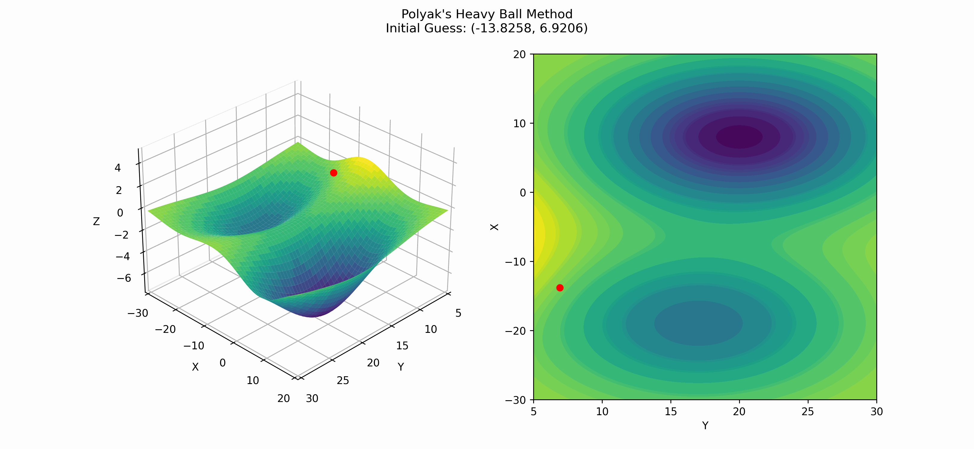
Again, we see that this method finds the local minima instead of the global minima, but it is interesting to note that as the slope of the surface changes, so does the distance between the more recent and current points. This is a result of the momentum parameter $\beta$.

Here is an example of when Polyak's heavy ball method finds the global minima.

One interesting thing about Polyak's method is that its convergence rate (for convex functions) is $\mathcal{O}(1/\sqrt{\varepsilon})$, where $\varepsilon$ is our tolerance threshold; meaning, if we want $$\lVert \textbf{x}_k - \textbf{x}^*\rVert$$ \leq \varepsilon,$$ we will need to run Polyak's method for $\mathcal{O}(1/\sqrt{\varepsilon})$ iterations. ($\textbf{x}^*$ is the true minimum of the function.)

Nesterov's Accelerated Gradient Descent Method

Another method that is similar to Polyak's Heavy Ball Method is Nesterov's Accelerated Gradient Descent Method. Nesterov's method is essentially advanced Polyak's method with a twist. A big part of Polyak's method over gradient descent is the idea of momentum. This momentum, however, can hurt us in the end as it can cause us to overshoot the minimum. Nesterov's method incorperates the idea of damping (or friction) into Newton's law of motion. If we write $$ma = F - cv,$$ where $m$ is the mass of the object, $a$ is the acceleration, $F$ is the force, $c$ is the damping coefficient, and $v$ is the velocity. In this, we have that the effective force helps to decrease the velocity of the object. This allows the weight updates to not slow down in the beginning when the gradient is large. However, as we get closer to the minimum and the gradient magnitude is smaller, the damping coefficient will help to slow down the weight updates and prevent overshooting.

To perform Nesterov's method, we can use the following update equations: $$\begin{aligned} \textbf{u}_{k+1} &= \beta\textbf{u}_k - Df(\textbf{x}_k + \beta\textbf{u}_k) \\ \textbf{x}_{k+1} &= \textbf{x}_{k+1} + \beta(\textbf{u}_{k+1}). \end{aligned} $$ It is important to point out that the only difference between this method and Polyak's method (at least the second alternative implementation) is the terms inside the derivative $Df$. This main change computes the gradient as if the weights have already moved with the current velocity $\textbf{u}_k$. It then uses that velocity to update the weights. An alternative way to write this update is $$\begin{aligned} \textbf{u}_{k+1} &= (1 + \beta)\textbf{x}_k - \beta\textbf{x}_{k-1} \\ \textbf{x}_{k+1} &= \textbf{u}_{k} - \alpha Df(\textbf{u}_{k}). \end{aligned}$$

The first way, implemented in Python, is given by

def nag(f, x0, alpha=0.1, beta=0.7, tol=1e-6, maxiter=10**5):
    # Get our initial guess
    x_vals = np.array([x0])
    x = x0
    v = np.zeros_like(x0)
    
    # Iterate until we converge
    for i in tqdm(range(maxiter)):
        # Get the gradient
        grad = opt.approx_fprime(x - beta*v, f, 1e-6)
        
        # Update our guess
        v_new = beta * v + alpha * grad
        x_new = x - v_new
        x_vals = np.vstack((x_vals, x_new))
        
        # Check for convergence
        if np.linalg.norm(x_new - x) < tol:
            break
        
        x = x_new
        v = v_new
        
    return x_vals, i

In this case, v_new is our $\textbf{u}_k$.

Applying this to our test function, we get

Nesterov's method hits the global minimum in this case, but it is very possible for Nesterov's to hit a local minima.

Other Gradient Descent Methonds

These methods discussed today are not the only methods for gradient descent. There are many other methods that have been developed over the years. Some of these methods include:

• Adagrad
• Adam
• Adadelta
• RMSprop
• LBFGS

but the current most popular method is Adam. I will touch on Adam in a future blog post.

Conclusion

Gradient descent is a huge, key component of deep learning and optimization. While not perfect, gradient descent does a dang good job for non-convex functions. Some of the main methods we covered today are standard gradient descent, Polyak's Heavy Ball Method, and Nesterov's Accelerated Gradient Descent. These methods all have their strengths and weaknesses, but they all have the same goal: to minimize a function. I hope you enjoyed this blog post. I invite you to check out the iPython notebook I used to write all the methods and create the graphs and animations (it took me a long time to figure out, so just take what I did and don't reinvent the wheel haha).