Introduction to Knot Theory: Slice Surfaces and Slice Genus
"Nobody can point to the fourth dimension, yet it is all around us."
- Rudy Rucker
Continuing on from my previous blog post, this blog post focuses on slice surfaces and the slice genus of a knot.
Introduction to Surfaces
In the results to follow, one important idea to understand is that of a topological surface (or simply a surface). A topological surface is a two-dimensional manifold, intuitively representing a flat, rubbery sheet that can be stretched, bent, and manipulated without tearing or gluing. Surfaces can be orientable, which simply means you can distinguish between the 'front' and 'back' of the surface.
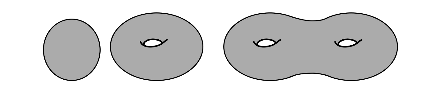
An important piece of information about an orientable surface is its genus. The genus of a surface is a fundamental topological invariant describing the shape and structure of the surface. Intuitively, it can be thought of as the number of "handles" or "holes" that a surface possesses (see Figure 2). Every orientable surface is topologically equivalent some surface with specified genus.
Seifert Surfaces
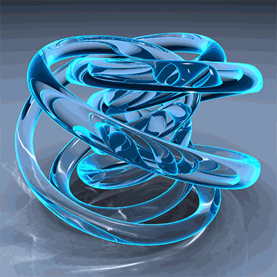
If we take an orientable surface and cut a hole in it, we then get a surface with boundary. Given a knot $K$, we can always find a surface with boundary whose boundary is the knot $K$ [1]. Such a surface is called a Seifert surface for K. More precisely, a Seifert surface is an oriented surface associated with a knot or link on its boundary in three-dimensional space (see Figure 3).
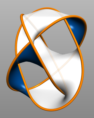
One of the ultimate goals of representing knots in this way is to find the simplest surface possible to represent a given knot, which is not always obvious. For example, the minimal genus of a Seifert surface bounded by a certain knot may be 3, but an explicit minimal genus surface might be difficult to find. Thankfully, the Seifert genus (which is defined as the minimal genus of a Seifert surface bounded by the knot) is relatively easy to calculate.
Slice Surfaces
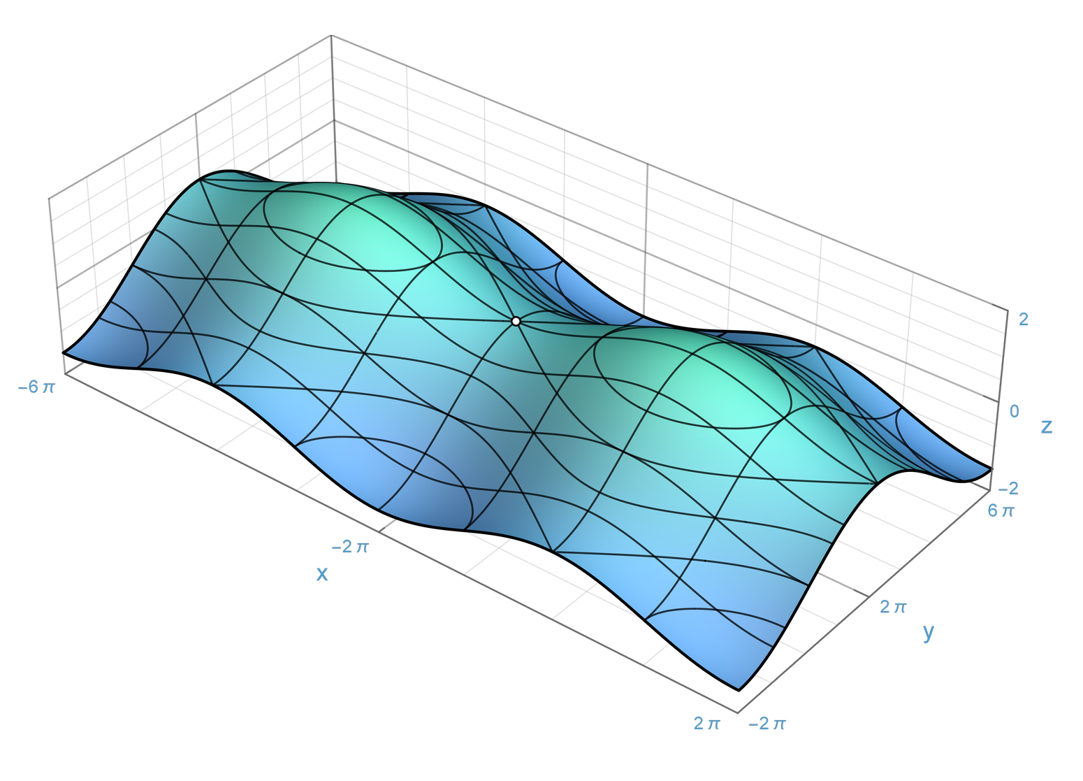
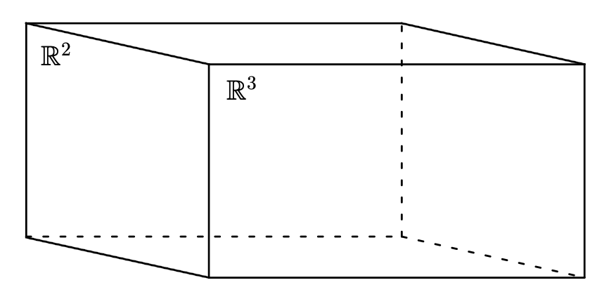
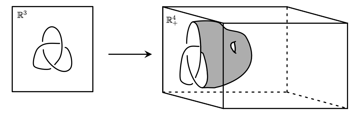
Now suppose that you have knot that bounds a surface in $\mathbb{R}^{3}$ of genus 2, but would like to construct a surface that it bounds with genus 1. One possible solution is that instead of requiring the surface to live entirely inside $\mathbb{R}^{3}$, we can allow it to dip into $\mathbb{R}^{4}$. Just as we can think of $\mathbb{R}^2$ being the boundary of $\mathbb{R}^3_+ = \{(x,y,z) \in \mathbb{R}^3 \, | \, z \geq 0 \}$ (see Figure 4), we can think of $\mathbb{R}^3$ as being the boundary of $\mathbb{R}^4_+= \{(x,y,z,t) \in \mathbb{R}^3 \, | \, t \geq 0 \}$. Given a knot $K$ in $\mathbb{R}^3$ we can therefore consider surfaces in $\mathbb{R}^4_+$ that are bounded by $K$. These surfaces that dip into $\mathbb{R}^{4}_+$ are called \emph{slice surfaces}, and the \emph{slice genus} of a knot is the minimal genus of any slice surface you can find for that knot (see Figure 5). Unfortunately, the slice genus is much more difficult to calculate than the Seifert genus.
Since visualizing $\mathbb{R}^{4}$ is quite difficult, representing slice surfaces can be a bit of a problem. One way to overcome this is by looking at level sets. Level sets are a way of representing a slice surface in $\mathbb{R}^4_+$ by taking a 'slice' out of the surface at various levels and seeing what the surface looks like at the location of the slice. One dimension lower, taking level sets of a surface in $\mathbb{R}^3$ yields a sequence of two-dimensional planes each containing a single slice of the surface. If you take enough of these level sets you will be able to get the full picture of the surface (see Figure 6).
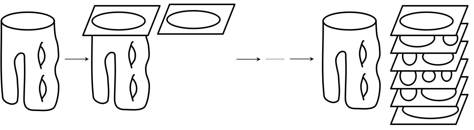
To take level sets in $\mathbb{R}^{4}$ we do the exact same thing as in $\mathbb{R}^{3}$. The only difference is now the level sets are each 3-dimensional slices with knots inside, instead of 2-dimensional planes with planar curves.
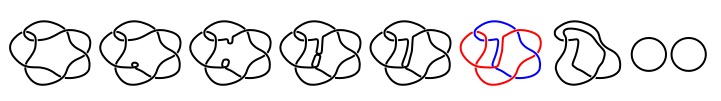
When studying the level sets of a slice surface in $\mathbb{R}^4_+$ there are a finite number of ways the level sets may change from one picture to another. If the surface has a \emph{saddle point} then passing the saddle point will change the level sets by bringing two nearby strands together and merging them (see the change that happens between the fourth and fifth diagrams in Figure 7 below). In this context, we define a saddle point to be a point on the surface where the curvature takes on both positive and negative values along different directions. If the surface has a local minimal point, then passing the mimimal point will result in a single circle being deleted from the level set (in Figure 7, the two circles in the final level set sit just above a pair of local maxima, and passing these maximum points results in the two circles being deleted from the level set). Likewise, if the surface has a local maximum point, then passing the maximum point results in a single circle being added to the level set.
Conclusion
In this blog post, we discussed the basics of Seifert and slice surfaces. Understanding surfaces, particularly topological surfaces and their properties, is crucial in various fields, including knot theory. Seifert surfaces provide a valuable tool for representing knots, offering insights into their structure and complexity. Moreover, slice surfaces offer another perspective, allowing us to explore the interaction between knots and higher-dimensional spaces. While calculating the slice genus may pose challenges, techniques such as examining level sets provide valuable insights into the nature of slice surfaces. By delving into these concepts, we uncover not only the intricacies of knots but also deepen our understanding of the underlying mathematical structures that govern them.
Citations
-
[1] Heinrich Seifert. Über das Geschlecht von Knoten. In: Mathematische Annalen 110 (1935), pp. 571–592. DOI: 10.1007/BF01448044.